Introduction
- Signal:function depending on some variable with physical meaning
- Image:continuous function
- 2 variables:\(xy\) coordinates
- 3 variables:\(xy\) + time(video)
- Brightness is usually the value of the function
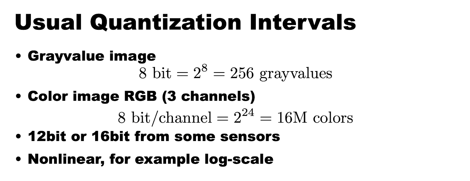
Geometric resolution:How many pixels per area;指图像中单位长度包含的像素或点的数目,常以像素/英寸(pixels per inch, ppi)度量。
Radiometric resolution:How many bits per pixel;指图像中可分辨的灰度级数目。
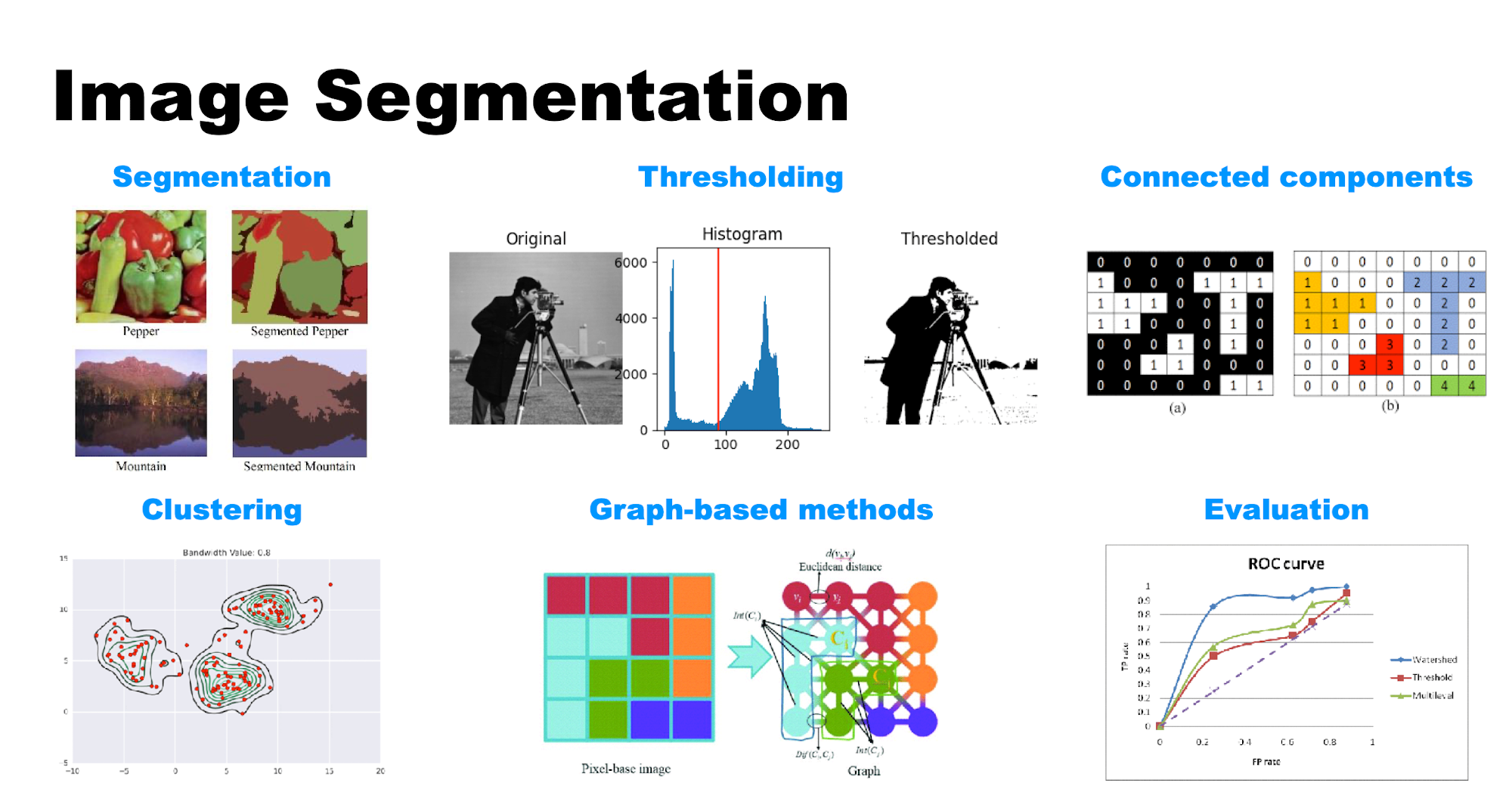
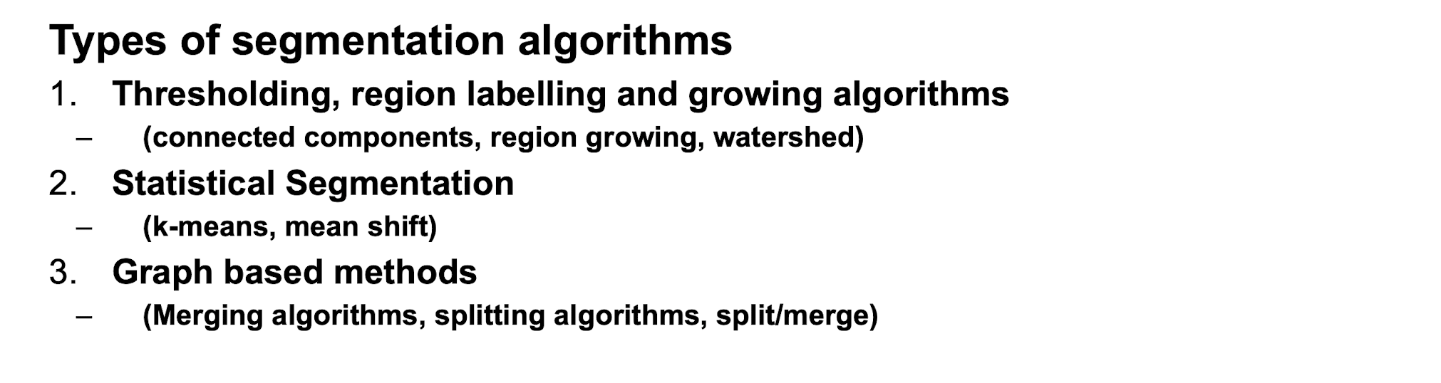
Segmentation
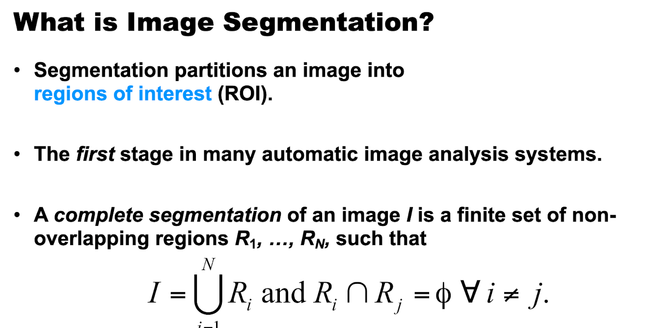
- 图像 \(I\) 可以表示为所有这些区域的并集 \(\bigcup_{i=1}^N R_i\)。
- 任意两个不同的区域 \(R_i\) 和 \(R_j\)(其中 \(i\neq j\))不相交,即 \(R_i\cap R_j=\emptyset\)。
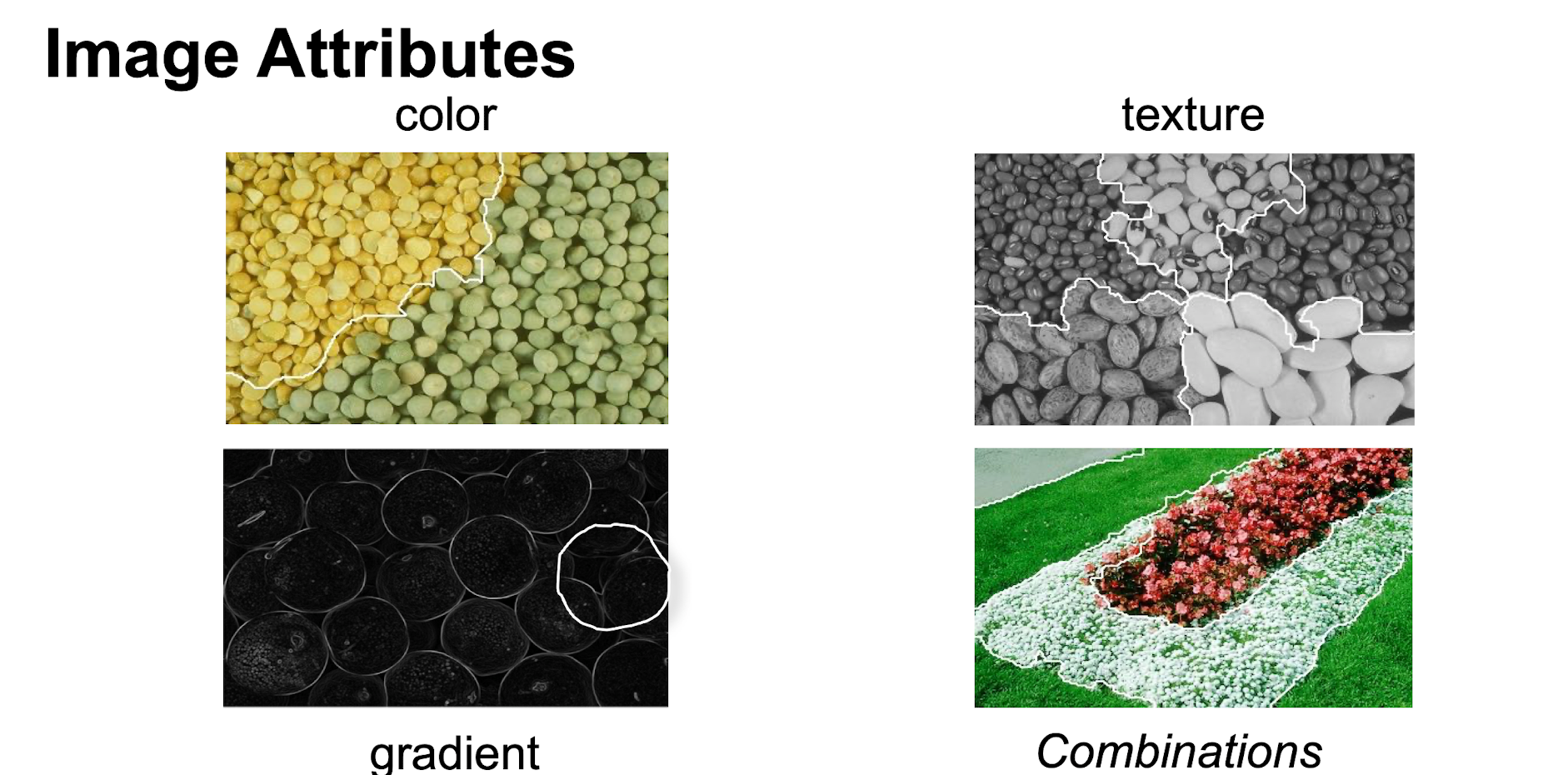
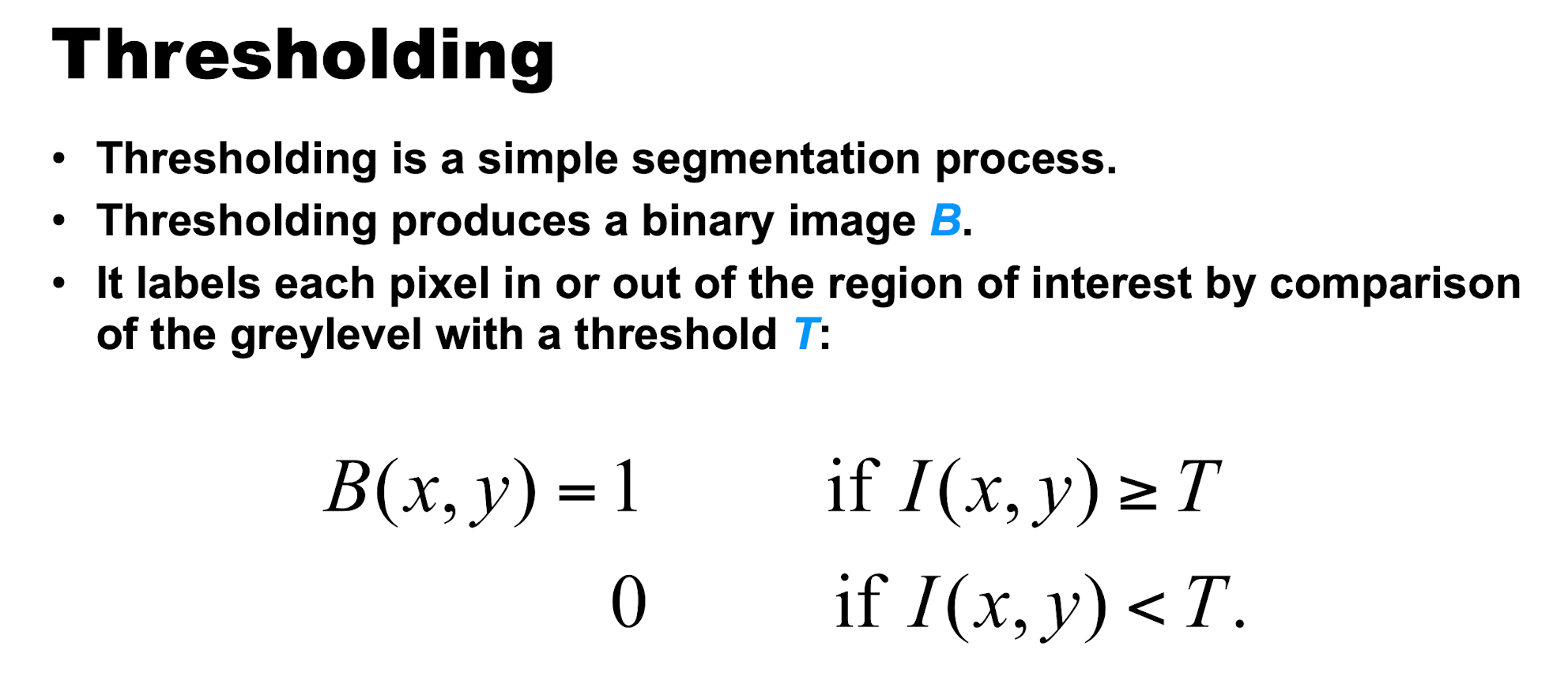
1. Thresholding、region labelling 与 region growing
ROC 曲线
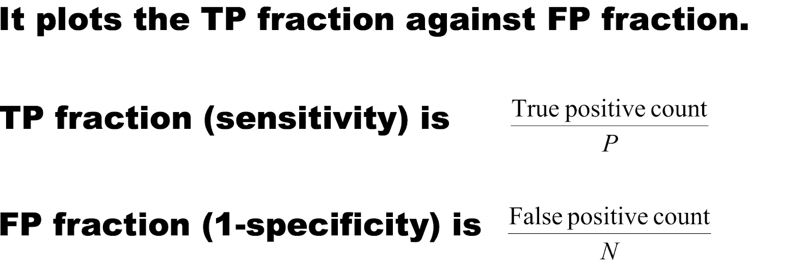
ROC(receiver operating characteristic)曲线刻画了一个二分类器的性能。二分类器用于区分两类事物,例如:
- Healthy / afflicted patients —— cancer screening
- Pregnancy tests
- Foreground / background image pixels
- Object detection

\[ \begin{aligned} TPR &= TP/P = TP/(TP+FN) \\ FPR &= FP/N = FP/(FP+TN) \end{aligned} \]
如果两类都服从高斯分布,曲线下面积可以直接算出来:
\[ A=Z\left(\frac{|\mu_P-\mu_N|}{\sqrt{\sigma_P^2+\sigma_N^2}}\right) \]
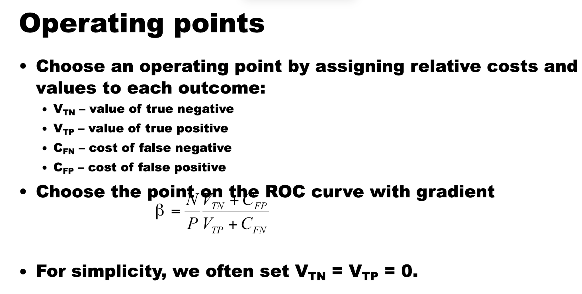
把真阳性的价值(\(V_{TP}\))和真阴性的价值(\(V_{TN}\))设为 0,这个简化假设基于一类特定场景:我们关心的是避免错误分类,而不是从正确分类中直接获益。在某些医学诊断或欺诈检测场景中,一个正确的分类可能没有直接的「奖励」,但一个错误的分类会带来成本或损失。
例如在疾病诊断中,真阳性(正确诊断为病人)可能没有额外的直接经济价值,因为它只是预期中的结果;但假阴性(错误地把病人诊断为健康)可能导致病情恶化,因此代价很高。同样,真阴性也可能没有额外价值,但假阳性(把健康个体诊断为病人)会导致不必要的焦虑和进一步的医疗检查,也带来成本。
Connected Components:Depth First
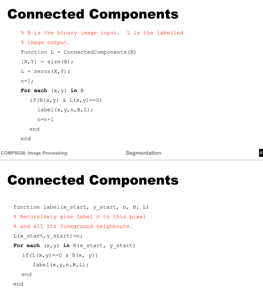
如果在位置 (x,y) 的 B 中的值是前景(逻辑值
1),并且在 L 中的相应位置还没有标签(即值为 0),则调用
label
函数,为这个像素及其所有相连的前景邻居像素递归地赋予当前标签
n。
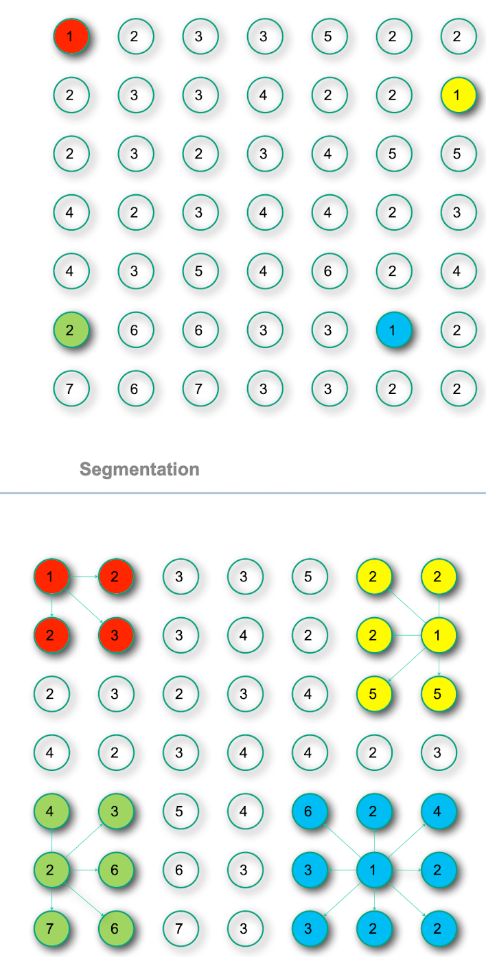
Region Growing:Breadth First
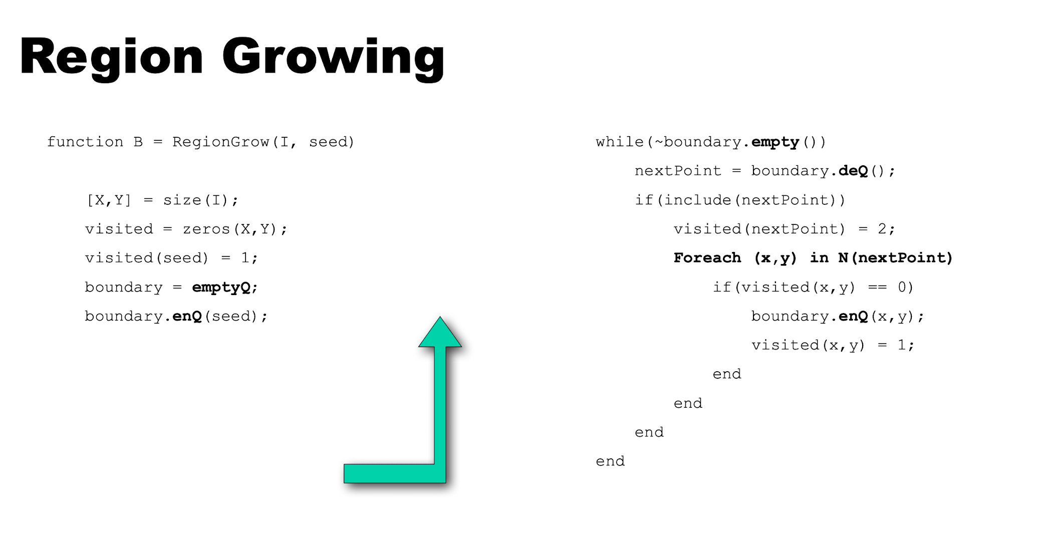
Seed:比如区域的亮度均值或中值。
Watershed Algorithm
Problem:watershed algorithm 通常会过分割(over-segment)。
Idea:用其他信息(如 cell nuclei)或手工标记来初始化区域,预先定义分割的数目。
三种方法的对比
Thresholding
- Relies on a single global threshold
- Produces separate regions(may prefer connected components)
Region growing
- Supervised,requires 1+ seed point
- Relies on a single threshold
- Produces one region
Watershed
- May be supervised or unsupervised
- No need for threshold parameter
- Partitions image into many regions
- To get good results, best to specify number and positions of seeds
2. Statistical Segmentation
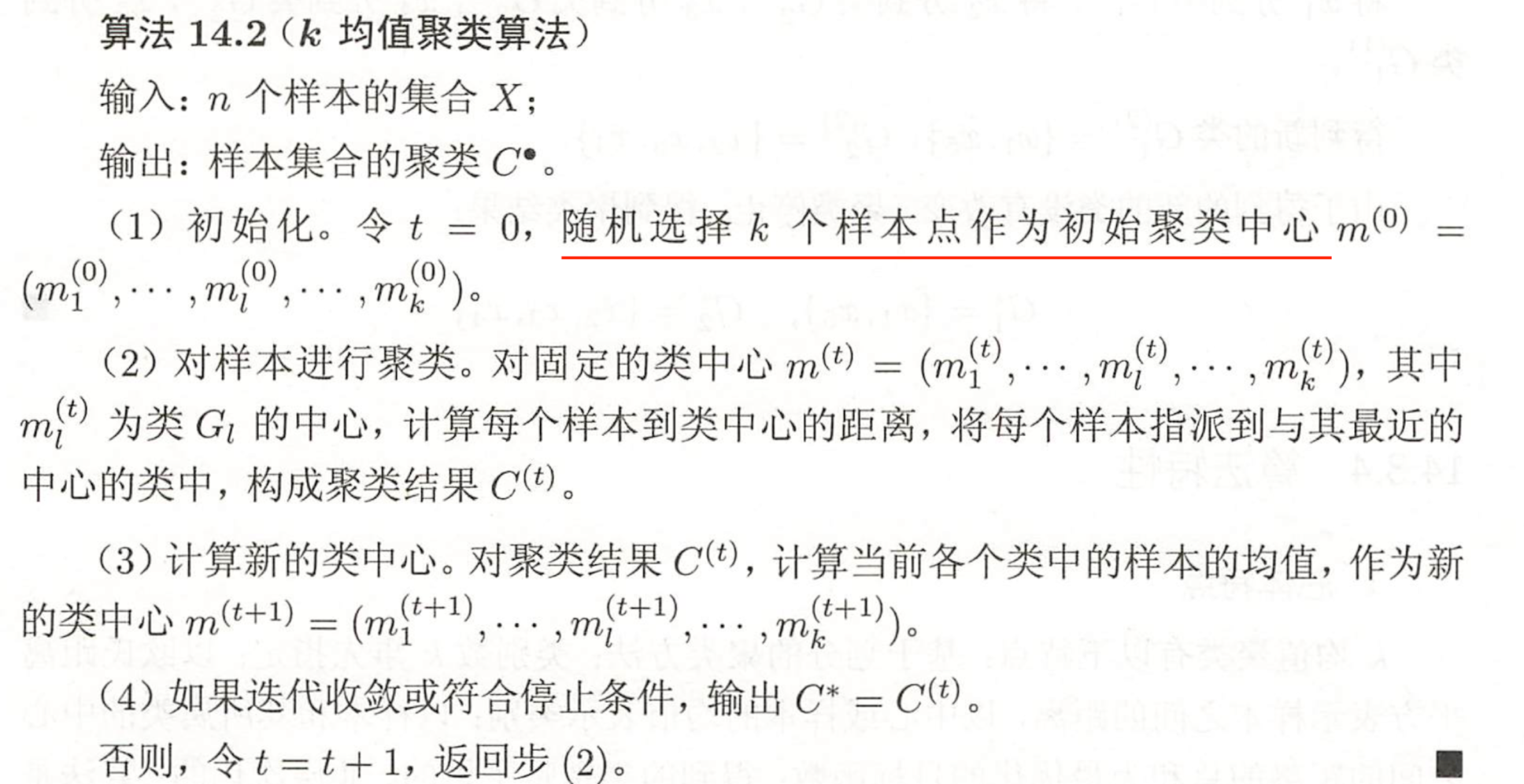
K-Means
Pros
- Simple and fast
- Converges to a local minimum of the distance function
Cons
- Need to pick \(K\)
- Sensitive to initialization
- Sensitive to outliers
- Only finds "spherical" clusters
Mean Shift
对每个样本构建以该样本为中心的高斯分布,累加所有高斯分布,就得到该数据集的密度。数据集密度的梯度方向就是密度增加最快的方向。
Pros
- Does not assume spherical clusters
- Just a single parameter(window size)
- Finds variable number of modes
- Robust to outliers
Cons
- Output depends on window size
- Computationally expensive
- Does not scale well with dimension of feature space
3. Graph-based methods
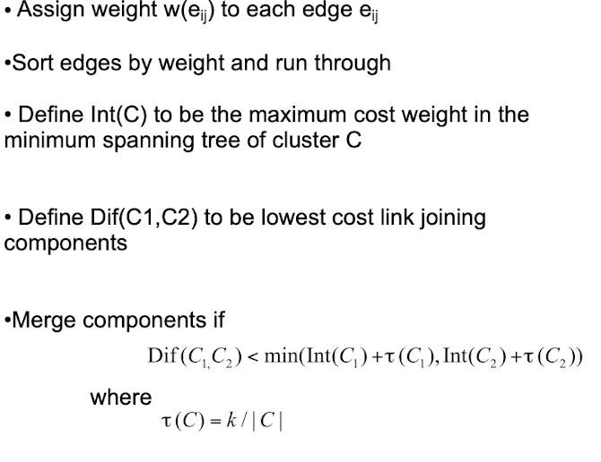
Merging algorithms
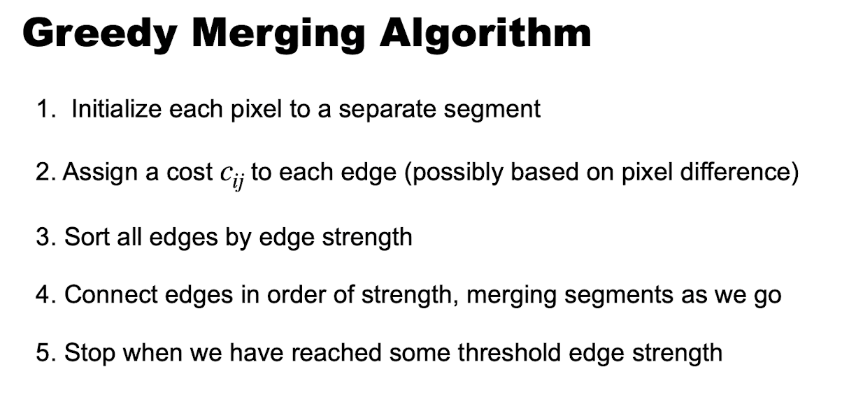
A better one:
Splitting Algorithm
计算 affinity matrix,然后对其做特征分解。
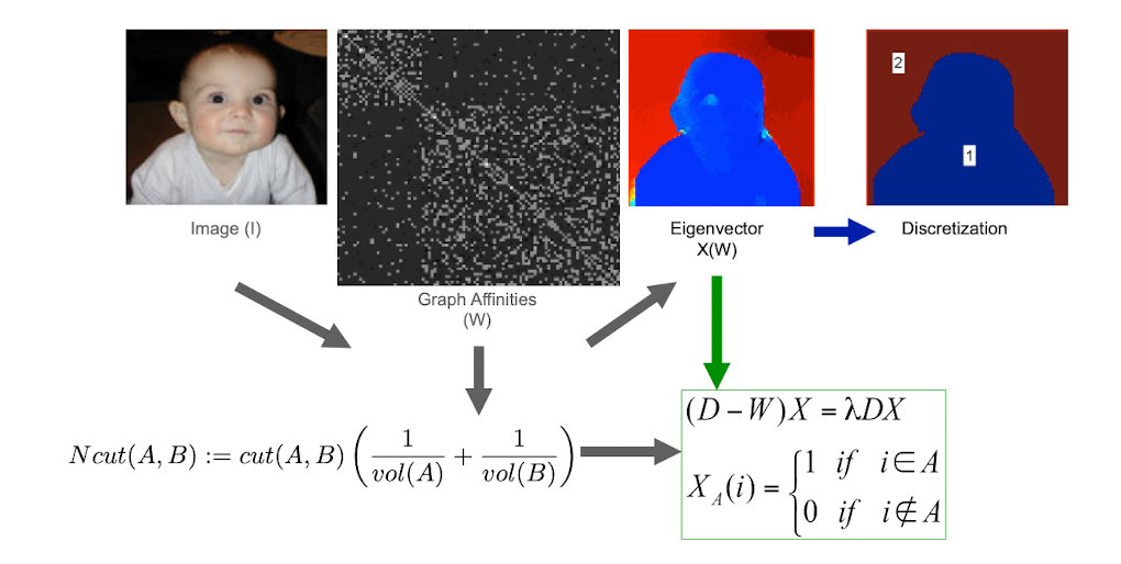
可以用 intensity、distance、texture 来构造 \(W\)。
使用 Normalized cut:
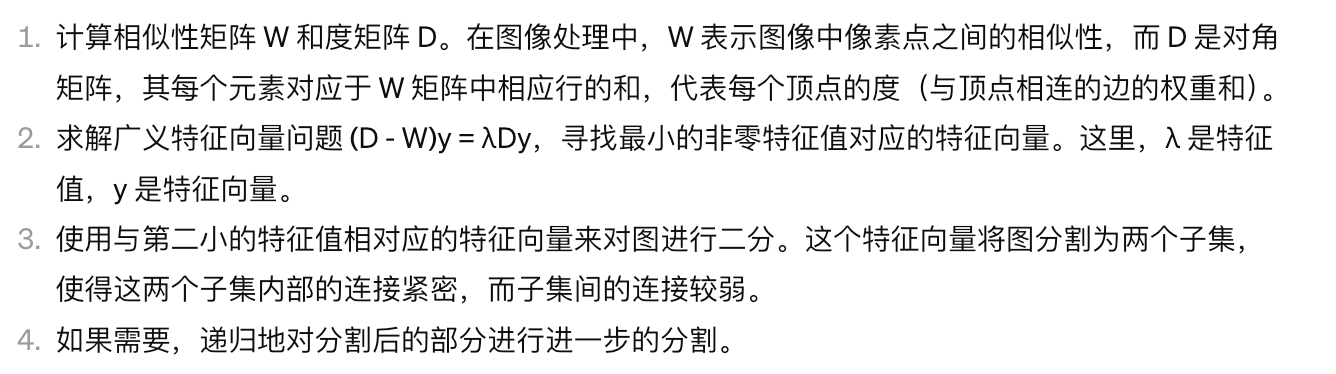
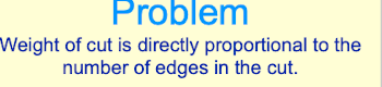
为什么不使用 Minimum cut?
Split and Merge Algorithms
Split:把图像看作一个整体区域,递归地检验区域是否满足同质性判据(例如区域内灰度方差小于阈值)。若不满足,就把该区域四等分(quadtree 划分),对每个子区域重复这一过程,直到所有区域都满足判据或达到最小尺寸。
Merge:划分结束后,相邻区域之间可能仍然同质。逐对检查相邻区域,若合并后的区域仍满足同质性判据,就把它们合并。反复迭代直到没有任何一对相邻区域可以再合并。
两步结合可以避免单纯 split 造成的过分割,也避免单纯 merge 对初始划分的敏感。
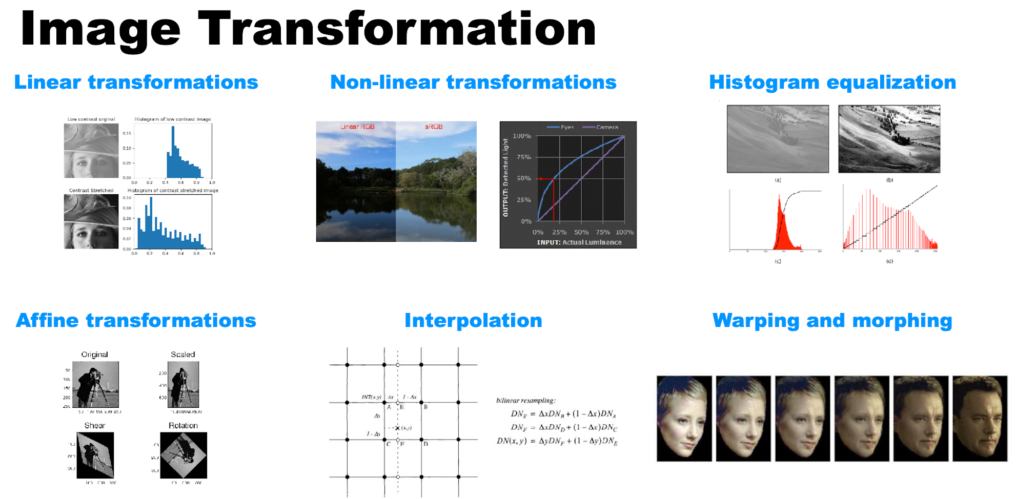
Transformation
Linear Transformation
\[ f(x) = \alpha x + \beta \]
Non-Linear Transformation
例如 gamma correction:
\[ f(x) = Ax^{\gamma} \]
其中 \(A = 255^{1-\gamma}\) 保证灰度范围不变。
- \(\gamma < 1\):more values for darker pixels
- \(\gamma > 1\):more values for brighter pixels
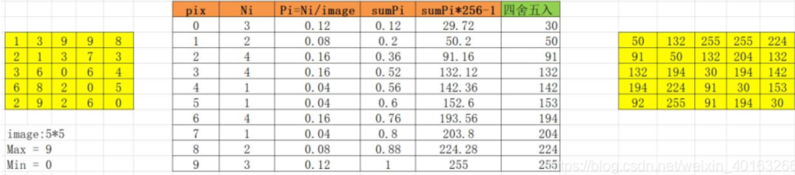
Histogram Equalization
Geometrical Transformation
改变图像特征的位置。
Affine transformation
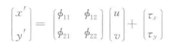
\(x',y'\) 是归一化相机坐标,\(u,v\) 是世界坐标系下某个平面上的点,共有 6 个自由度。
Interpolation
用周围位置插值来估计 \(I_1(x',y')\)。
Polynomial Warps
\[ \begin{aligned} x^{\prime}&=a_0+a_1x+a_2y+a_3x^2+a_4xy+a_5y^2 \\ y^{\prime}&=b_0+b_1x+b_2y+b_3x^2+b_4xy+b_5y^2 \end{aligned} \]
至少需要 6 对点。
Image Morphing
详见 Coursework 1。
Filtering
Filter:Let Intensity Through Selectively
Spatial Domain
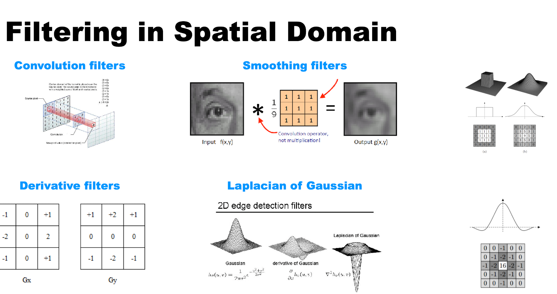
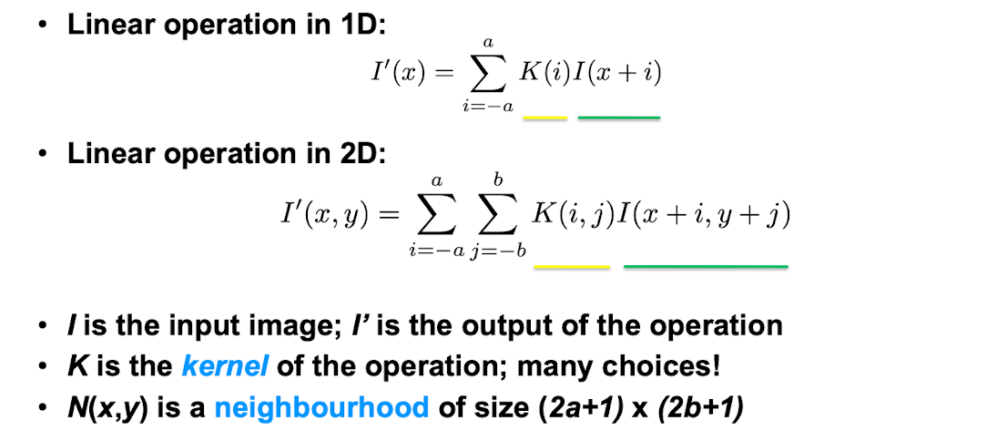
Correlation / Convolution
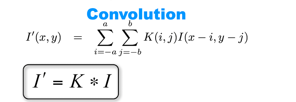
Filters
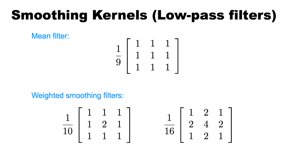
1. Low-pass filters(也叫 box filter)
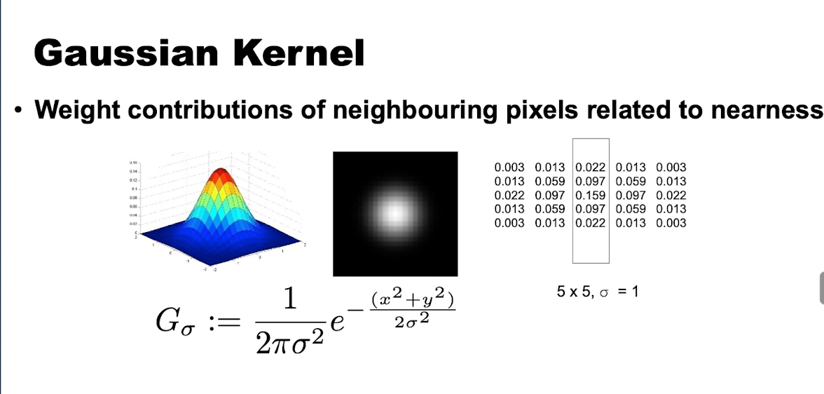
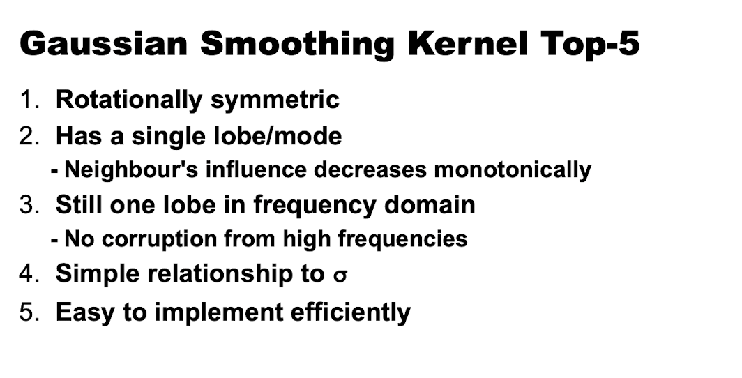
2. Gaussian Kernel
高斯函数的傅立叶变换仍然是高斯函数。
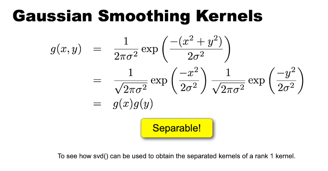
3. Separable Kernels
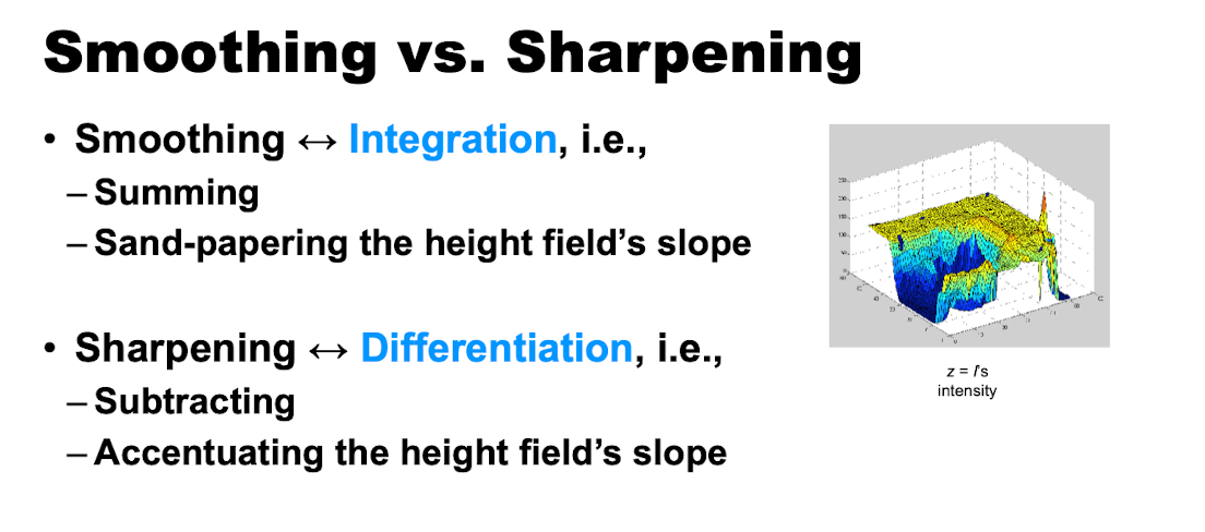
4. Smoothing vs. Sharpening
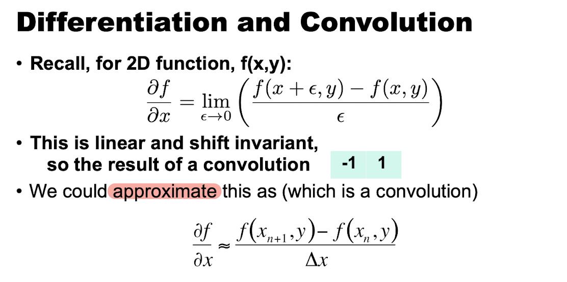
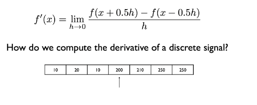
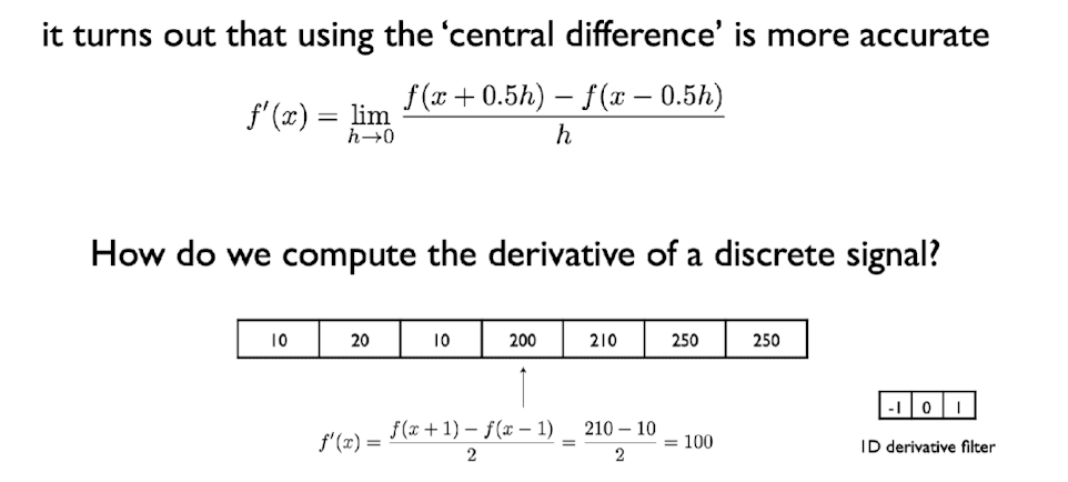
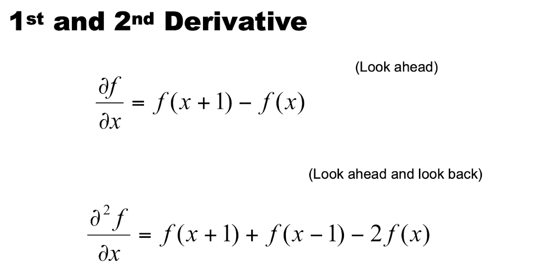
5. Differentiation and Convolution
6. Differential Filters
Prewitt 和 Sobel 都是一阶滤波器。
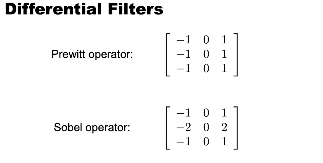
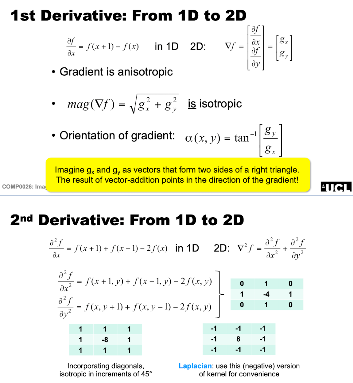
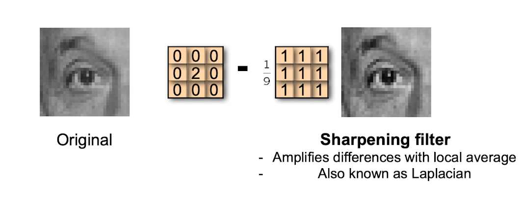
Image Sharpening
Laplacian operator 是 high-pass filter。
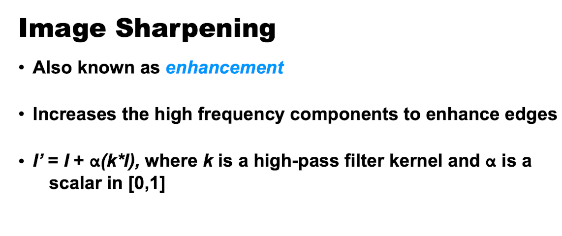
也可以写成 \(I' = I + \alpha(I - K * I)\)。
一个用于检测水平边缘的滤波器,可能在垂直方向上具有变化,而在水平方向上相对一致。这样在应用该滤波器时,它会高亮图像中的水平边缘区域,因为在那些区域图像与滤波器之间的点积会更大。
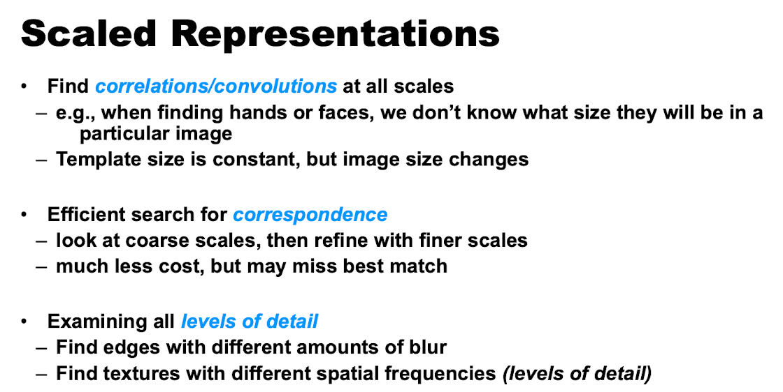
Scaled Representations
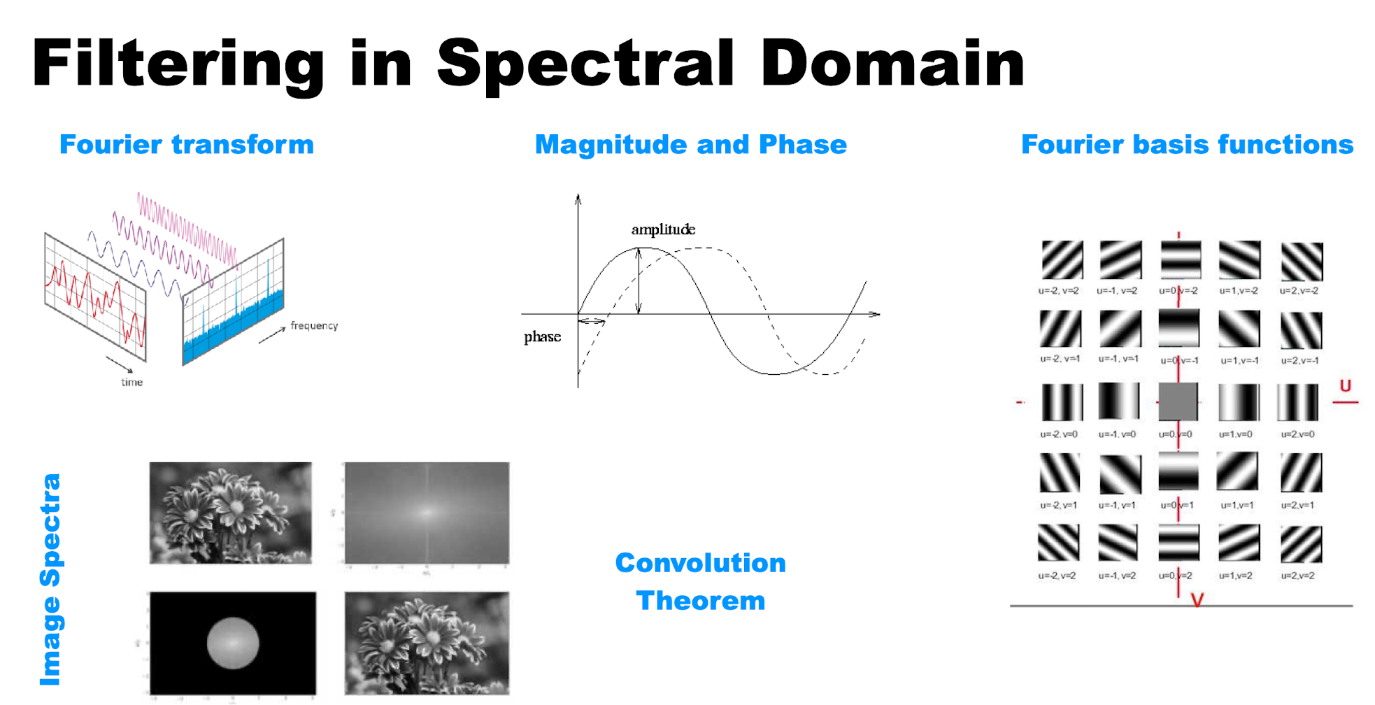
Fourier Domain
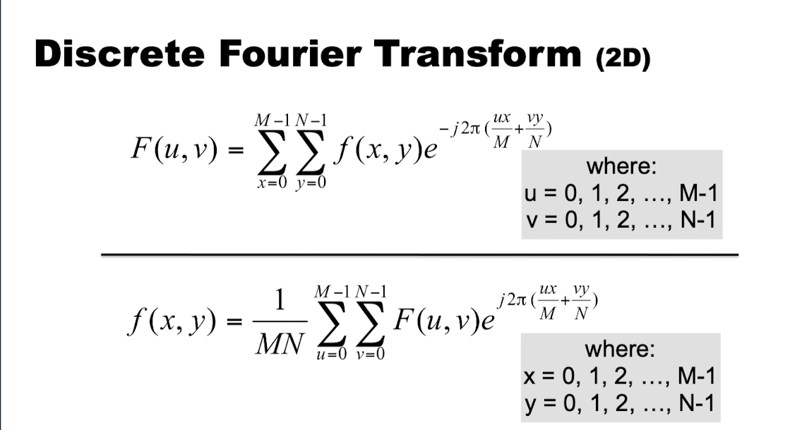
Fourier 域用加权频率分量之和来表示图像。许多图像处理操作在 Fourier 域中更简单,卷积在 Fourier 域中也更简单。
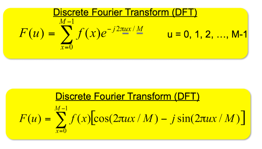
Fourier Series:任何周期函数都可以表示为一组正弦和余弦(基频的整数倍谐波)的加权和,其频谱是离散的。
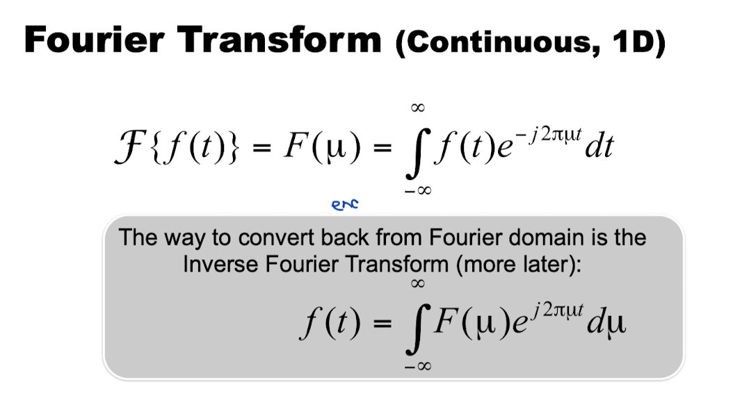
Fourier Transform:把上述结论推广到非周期函数——非周期函数可以表示为对连续频率的积分,其频谱是连续的。
Curious things about FT on images
- The magnitude spectra of all natural images are similar
- Heavy on low frequencies
- Falling off in high frequencies
- Most information in the image is carried in the phase, not the
amplitude
- Not quite clear why
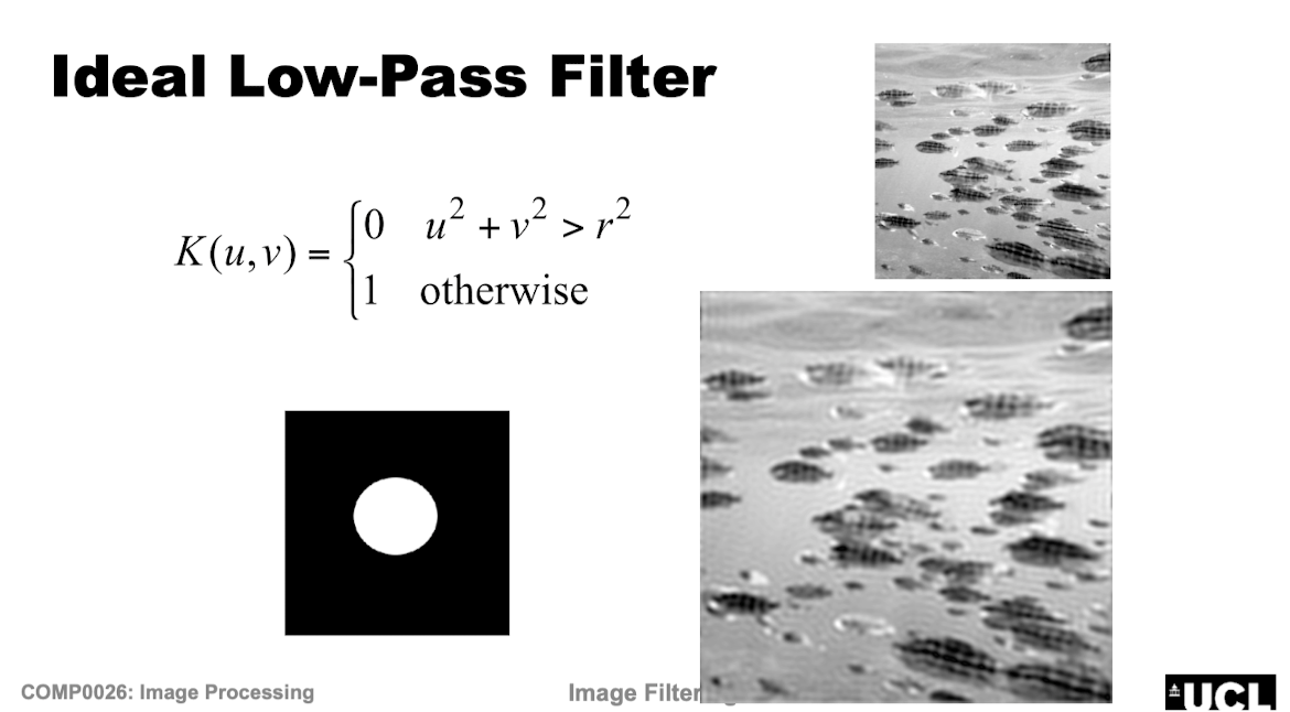
Ideal Low-Pass Filter
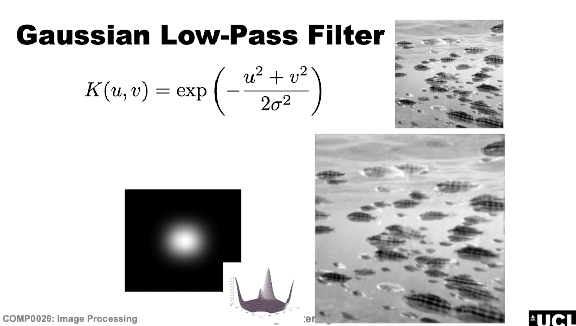
Gaussian Low-Pass Filter
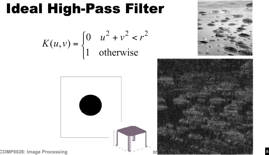
Ideal High-Pass Filter
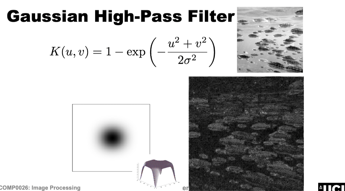
Gaussian High-Pass Filter
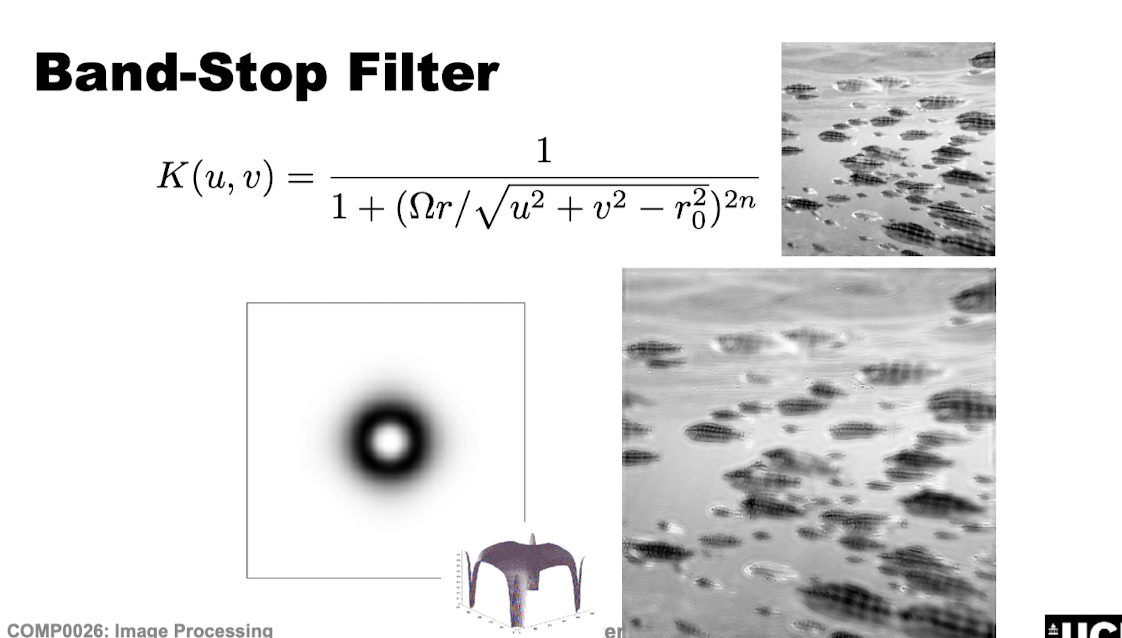
Band-Stop Filter
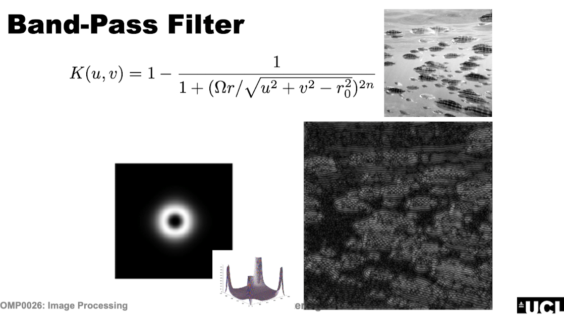
Band-Pass Filter
Order-statistic filters
Max Filter
\[ I^{\prime}(m,n)=\max\{I(i,j):(i,j)\in N(m,n)\} \]
Min Filter
\[ I^{\prime}(m,n)=\min\{I(i,j):(i,j)\in N(m,n)\} \]
Median Filter
\[ I^{\prime}(m,n)=\operatorname{median}\{I(i,j):(i,j)\in N(m,n)\} \]
Range Filter
\[ I'(m,n)=\max\{I(i,j):(i,j)\in N(m,n)\}-\min\{I(i,j):(i,j)\in N(m,n)\} \]
Rank Filters
基于邻域内灰度值排序的简单非线性滤波器:把邻域内的像素值从小到大排序,取第 \(k\) 个序统计量作为输出。上面的 max、min、median 都是 rank filter 的特例(分别取最大、最小、中位)。
Summary
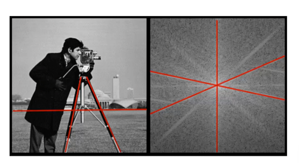
Edge Detection
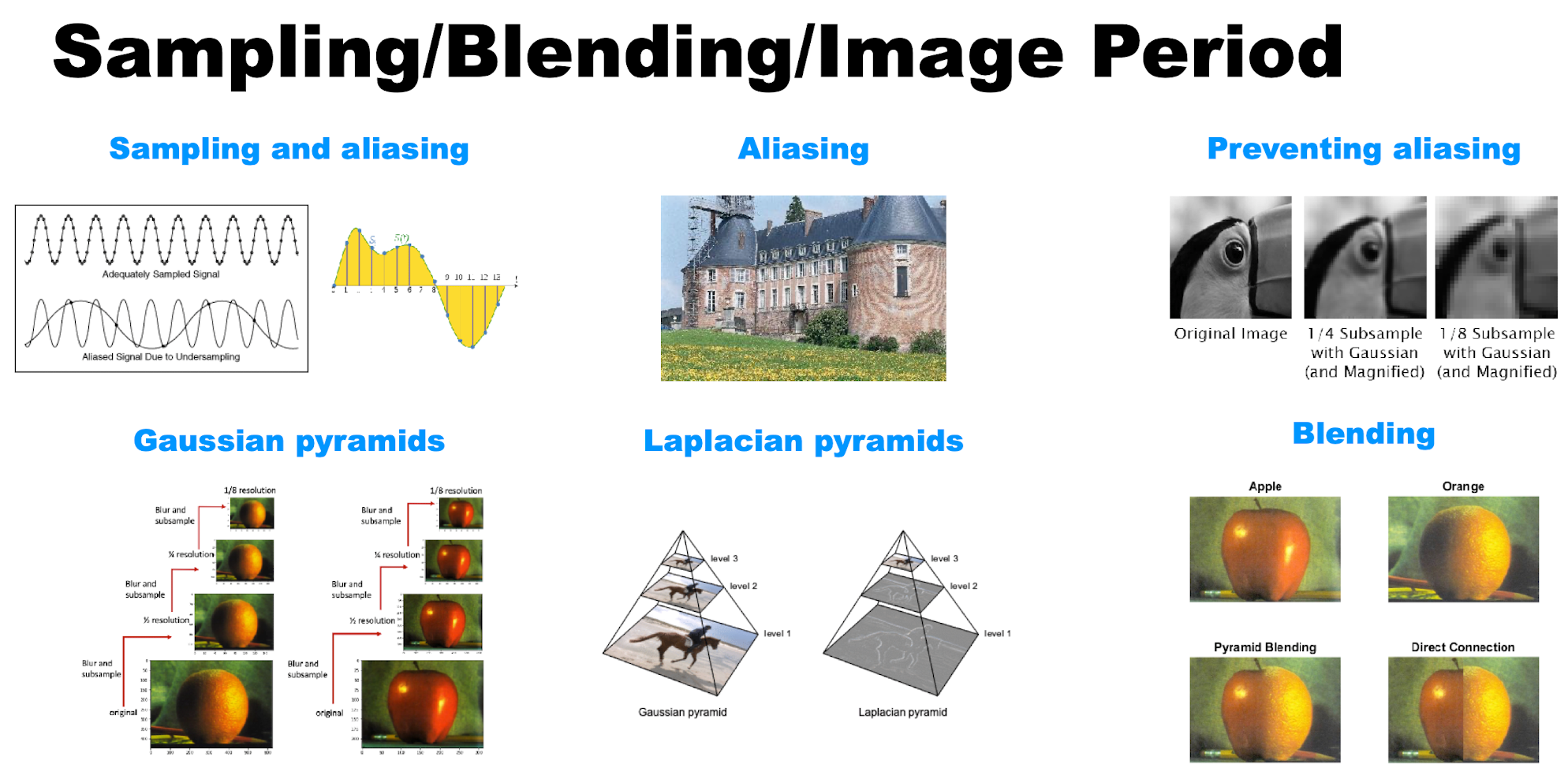
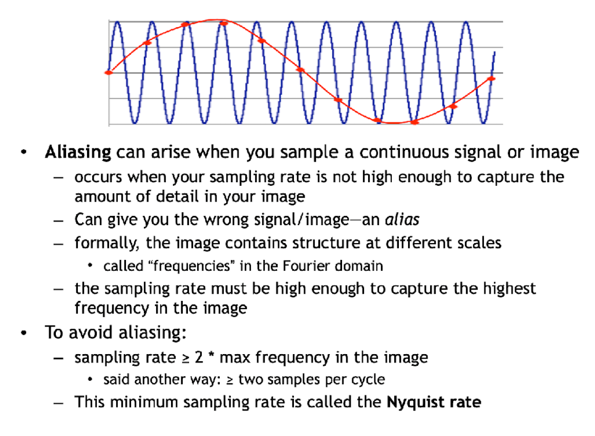
Aliasing
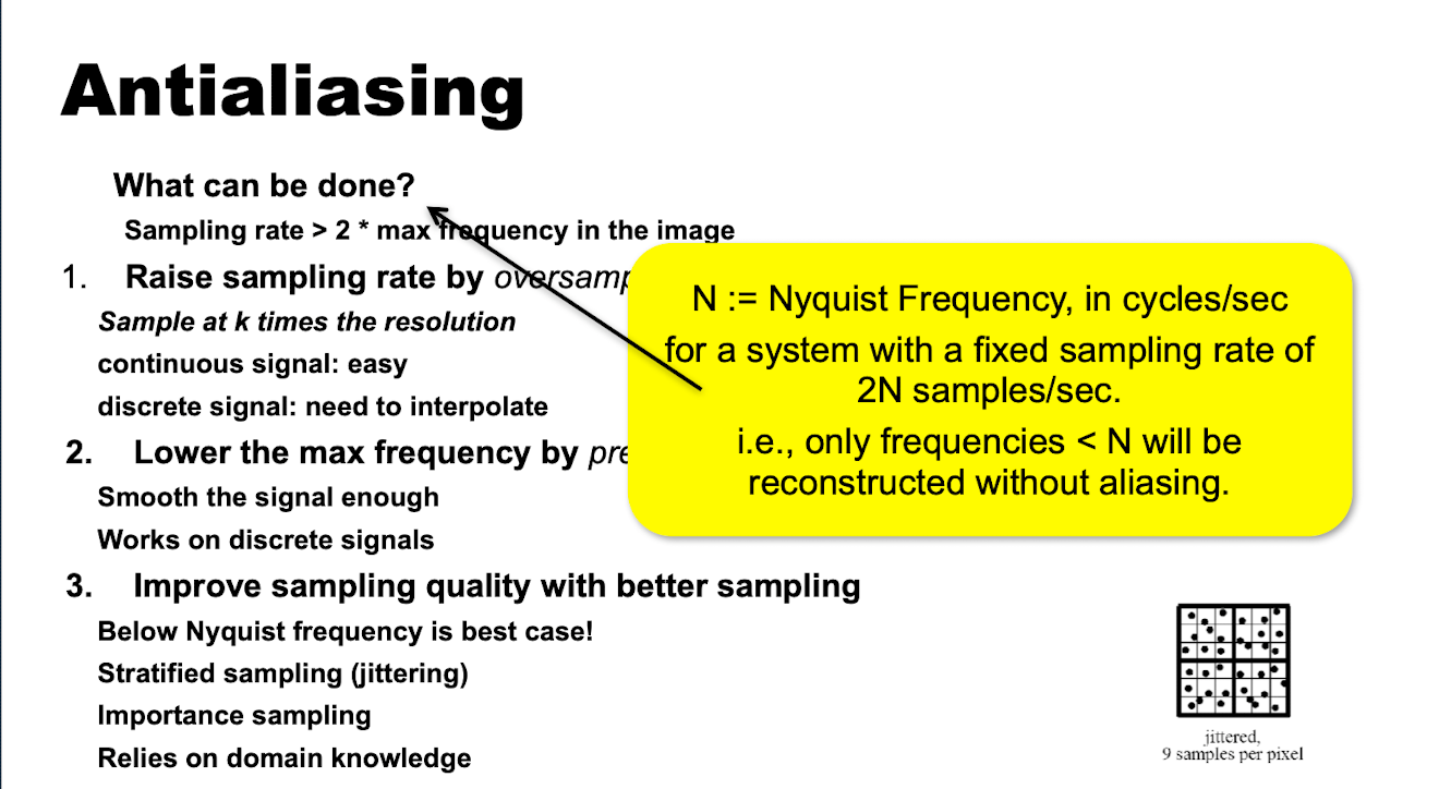
Sub-sampling
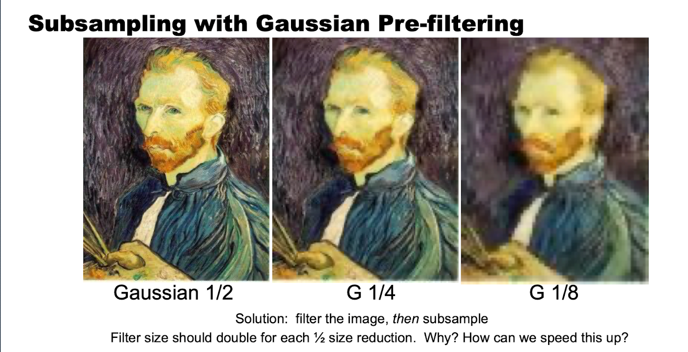
当图像被下采样或缩小时,高频内容变得更密集。如果不先用更大的滤波器平滑就直接下采样,可能会导致走样(摩尔纹效应)。
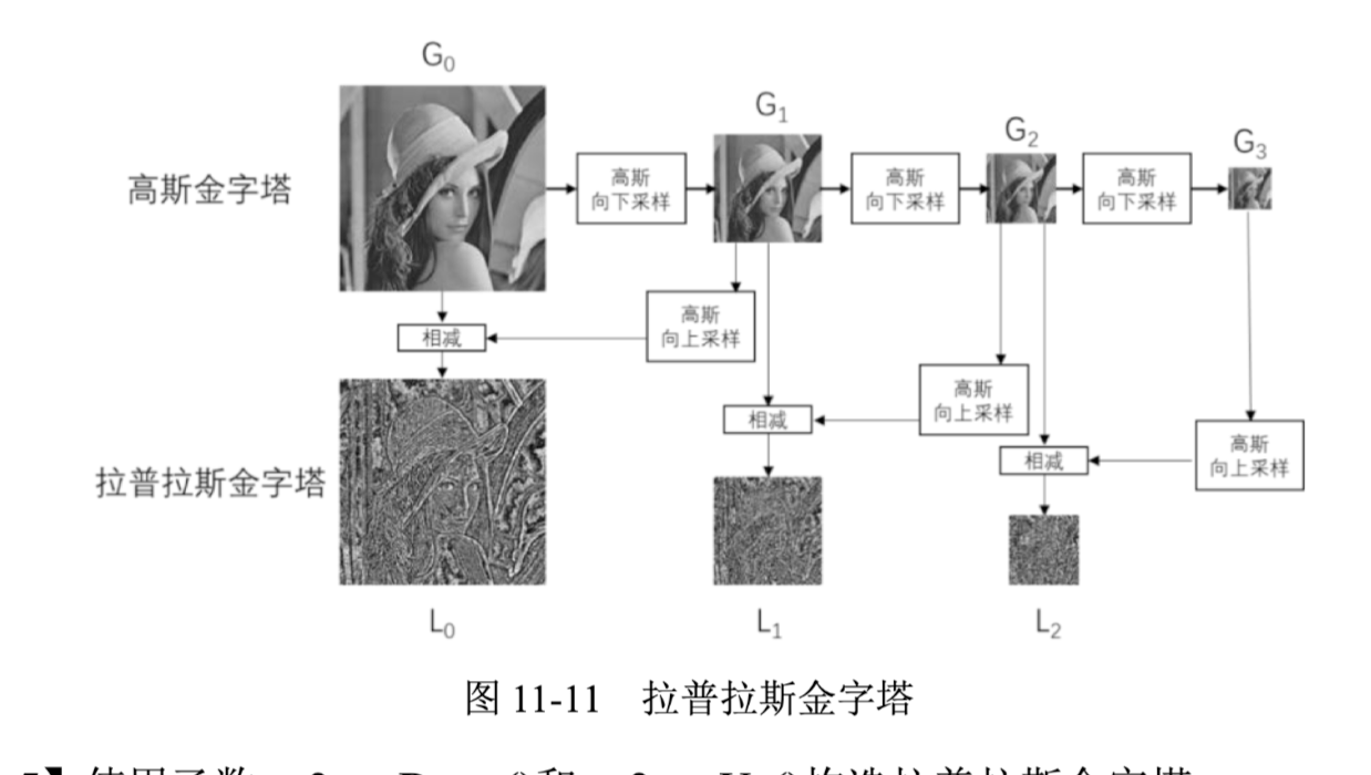
对一幅图像先上采样再下采样,是无法恢复其原始状态的;反之先下采样再上采样也一样。为了在上采样时能够恢复较高分辨率的原始图像,就要获取采样过程中丢失的信息——这些丢失的信息构成了拉普拉斯金字塔。
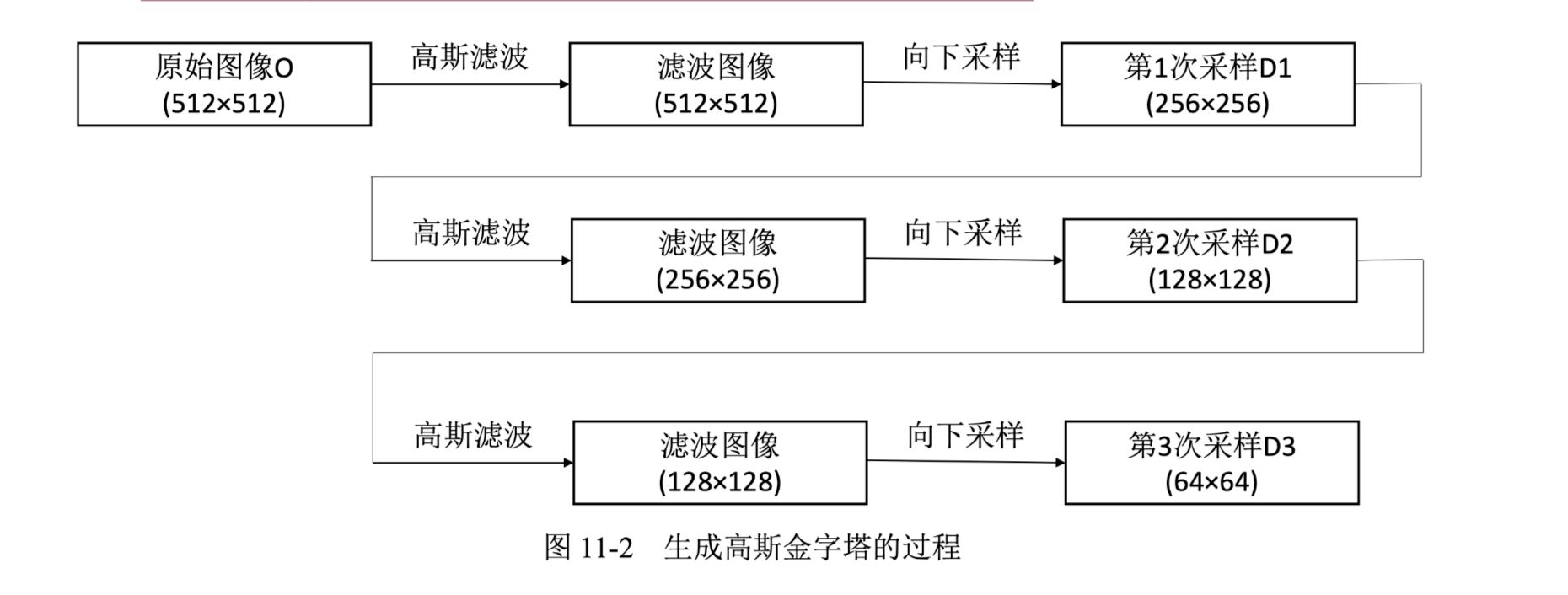
Gauss Pyramid
Laplacian Pyramid
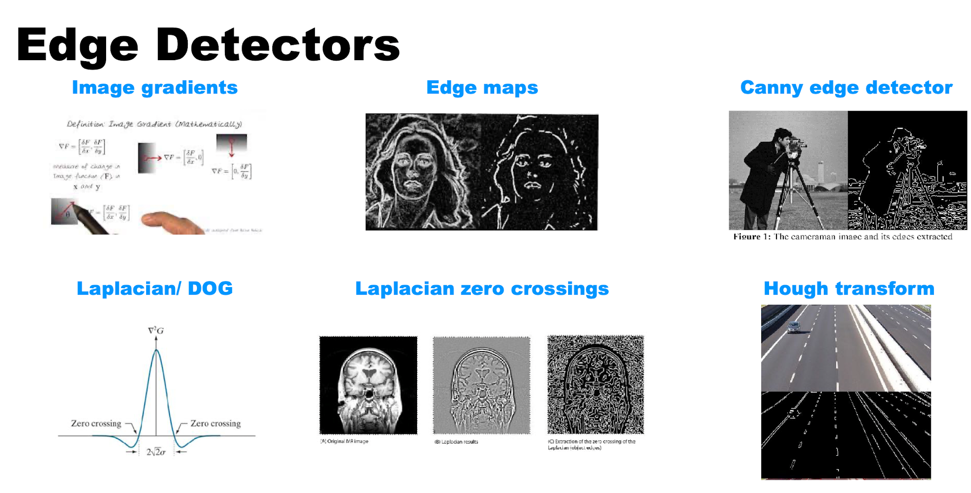
什么是边缘
Discontinuity of grey scale values。
Canny edge detector
- Smooth input image with Gaussian
- Compute gradient image:等价于与高斯的导数做卷积
- Apply non-maximal suppression
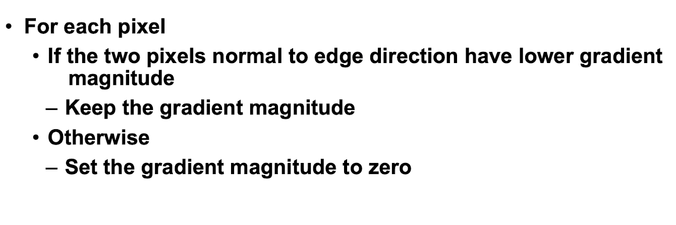
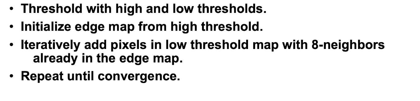
- Double thresholding(Hysteresis Threshold)
Marr-Hildreth Edge Detector
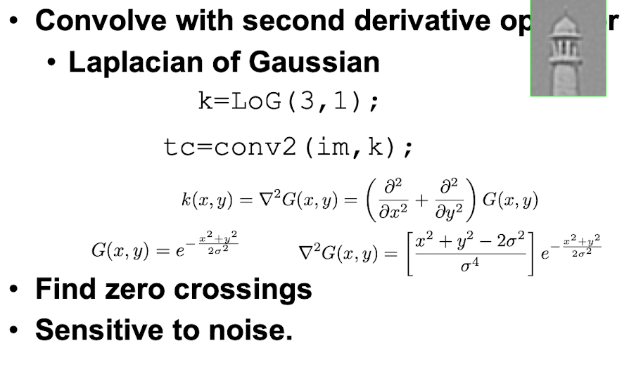
LoG(高斯拉普拉斯函数)
\[ \nabla^2G(x,y) = \left(\frac{x^2+y^2-2\sigma^2}{\sigma^4}\right)e^{-\frac{x^2+y^2}{2\sigma^2}} \]
尽管一阶导数可用于检测灰度突变,但它们是方向性算子。另一方面,拉普拉斯有着各向同性(旋转不变)的重要优点。
Marr-Hildreth:
\[ \begin{aligned} g(x,y)&=[\nabla^2G(x,y)]\bigstar f(x,y) \\ \text{等价于}\quad g(x,y)&=\nabla^2[G(x,y)\bigstar f(x,y)] \end{aligned} \]
DoG(高斯差分)
可以用 DoG 来近似 LoG:
\[ D_G(x,y)=\frac{1}{2\pi\sigma_1^2}\mathrm{e}^{-\frac{x^2+y^2}{2\sigma_1^2}}-\frac{1}{2\pi\sigma_2^2}\mathrm{e}^{-\frac{x^2+y^2}{2\sigma_2^2}} \]
Hough Transform
在霍夫坐标系内,经过一个点的线越多,说明其映射在极坐标系内的直线是由越多的点所构成(穿过)的。因此,霍夫变换检测直线的基本思路是:选择由尽可能多条线汇成的点。
通常做法是设置一个阈值,当霍夫坐标系内交于某点的曲线数量达到阈值,就认为在对应的极坐标系内检测到了一条直线。
上面讨论的是检测直线。实际上,只要是能够用一个参数方程表示的对象,都适合用霍夫变换来检测。
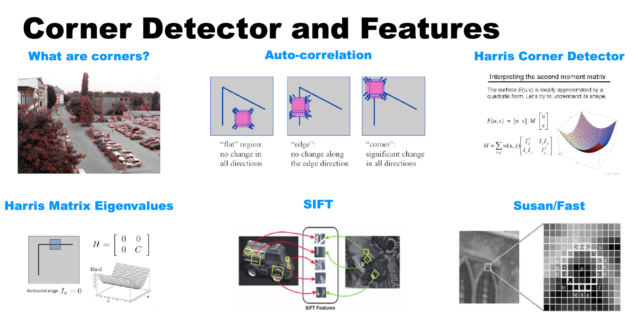
Corner Detector
Harris Corner Detector
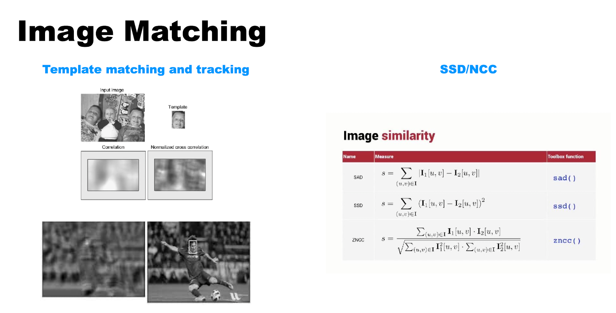
Motivation:Patch Matching
Intuition:一个好的匹配 patch 应该非常有区分度——在第二帧中只有一个 patch 看起来与它相似。
Corners:在该点邻域内,沿所有方向都有较大变化。
Basic idea:把窗口沿任意方向移动,都应该产生较大的外观变化。
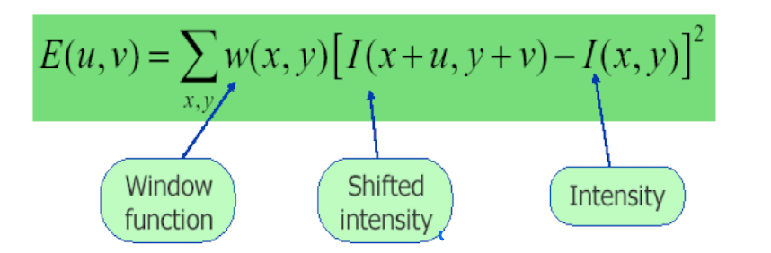
对于近似恒定的 patch,\([I(x+u, y+v) - I(x,y)]\) 会接近 0;而对于区分度很高的 patch,这个值会更大。
一阶近似:
\[ f(x+u,y+v)\approx f(x,y)+uf_x(x,y)+vf_y(x,y) \]
代入后展开:
\[ \sum[I(x+u,y+v) - I(x,y)]^2 = \begin{bmatrix}u&v\end{bmatrix} \left(\sum\begin{bmatrix}I_x^2&I_xI_y\\I_xI_y&I_y^2\end{bmatrix}\right) \begin{bmatrix}u\\v\end{bmatrix} \]
\[ E(u,v)\cong\begin{bmatrix}u&v\end{bmatrix}M\begin{bmatrix}u\\v\end{bmatrix}, \qquad M = \sum_{x,y}w(x,y)\begin{bmatrix}I_x^2&I_xI_y\\I_xI_y&I_y^2\end{bmatrix} \]
\(M\) 经过特征分解后等价于对角形式:
\[ M=\begin{bmatrix}\sum I_x^2&\sum I_xI_y\\\sum I_xI_y&\sum I_y^2\end{bmatrix} \sim\begin{bmatrix}\lambda_1&0\\0&\lambda_2\end{bmatrix} \]
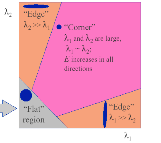
据此分类:
- 两个特征值都小:flat
- 一个大一个小:edge
- 两个都大:corner
通过特征值分类:
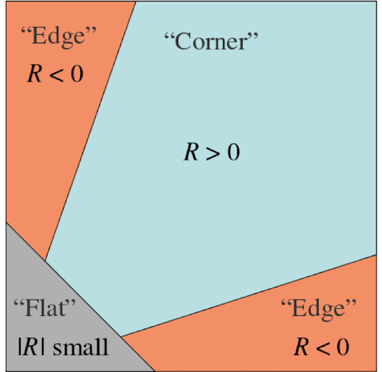
通过 \(R\) 分类:
\[ R = \det M - k(\operatorname{trace} M)^2, \qquad \det M = \lambda_1 \lambda_2, \qquad \operatorname{trace} M = \lambda_1 + \lambda_2 \]
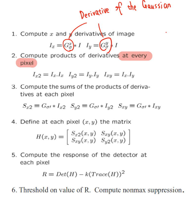
Workflow
- Compute corner response \(R\)
- Find points with large corner response:\(R > \text{threshold}\)
- Non-maxima suppression
Properties
- Invariant to rotations:椭圆会旋转,但它的形状(即特征值)保持不变
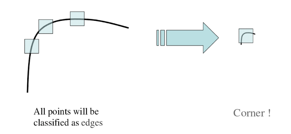
- Not invariant to image scale
SIFT Detector and Descriptor
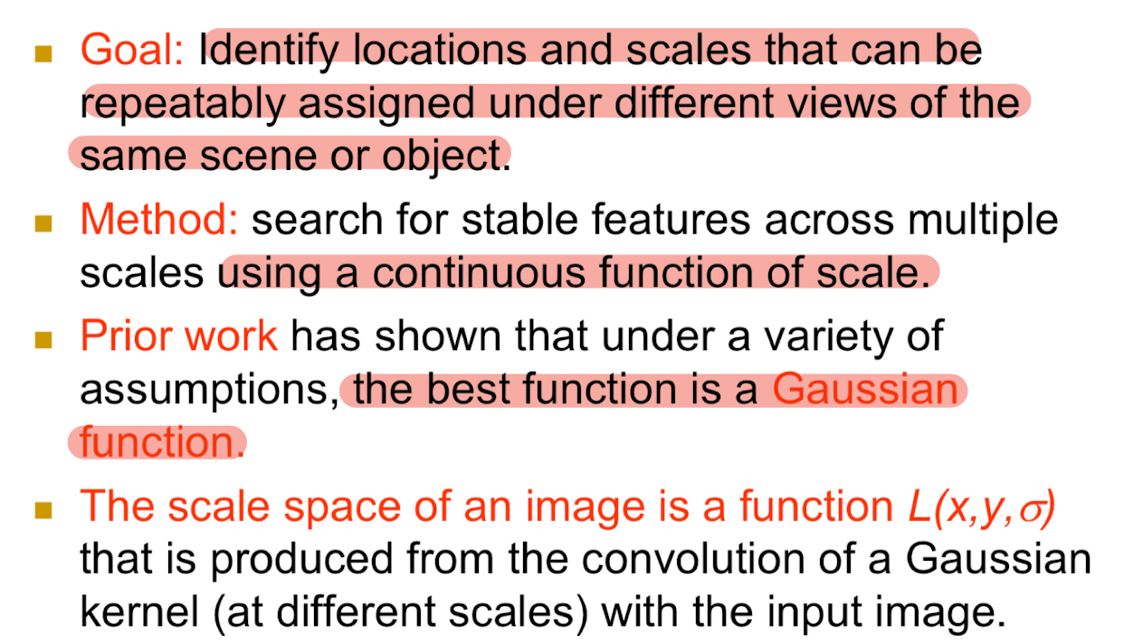
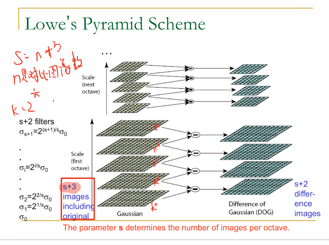
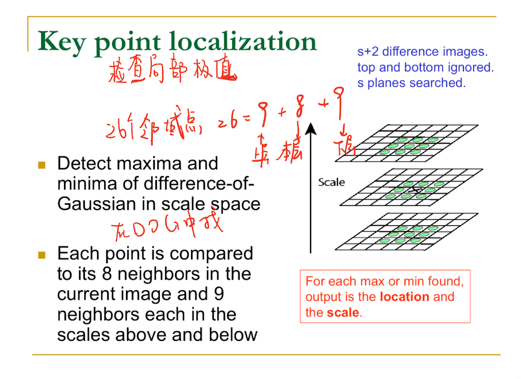
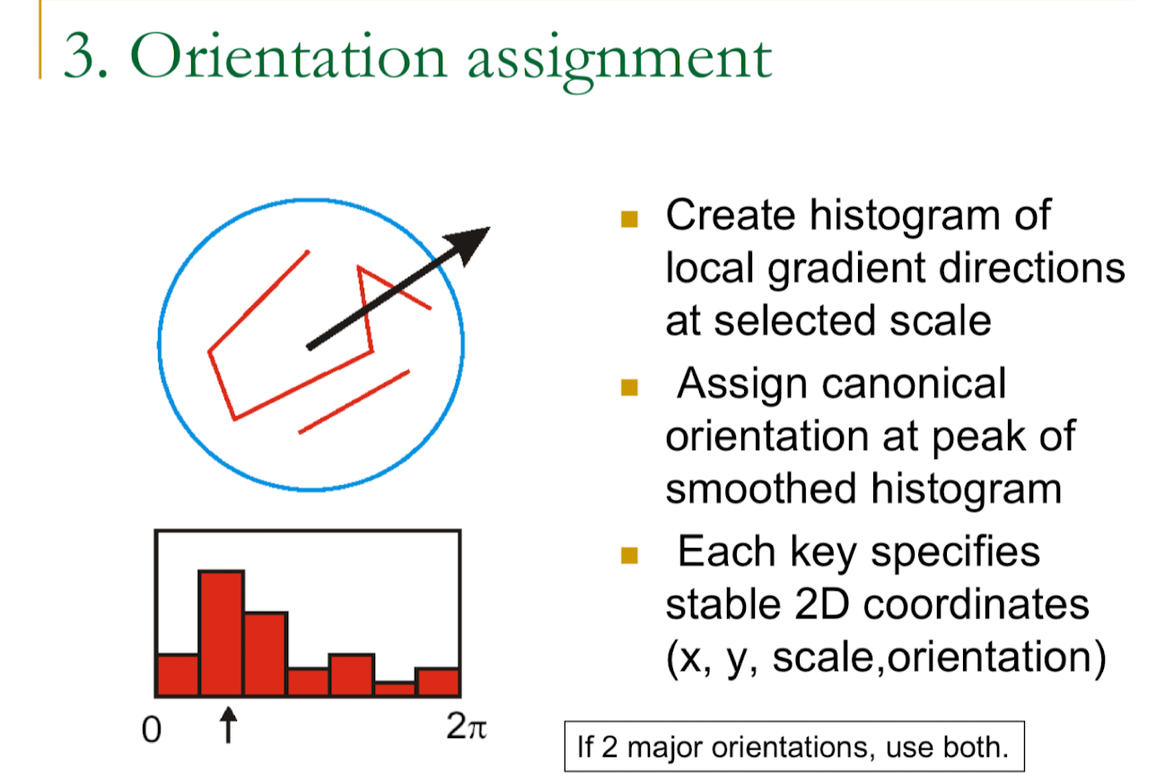
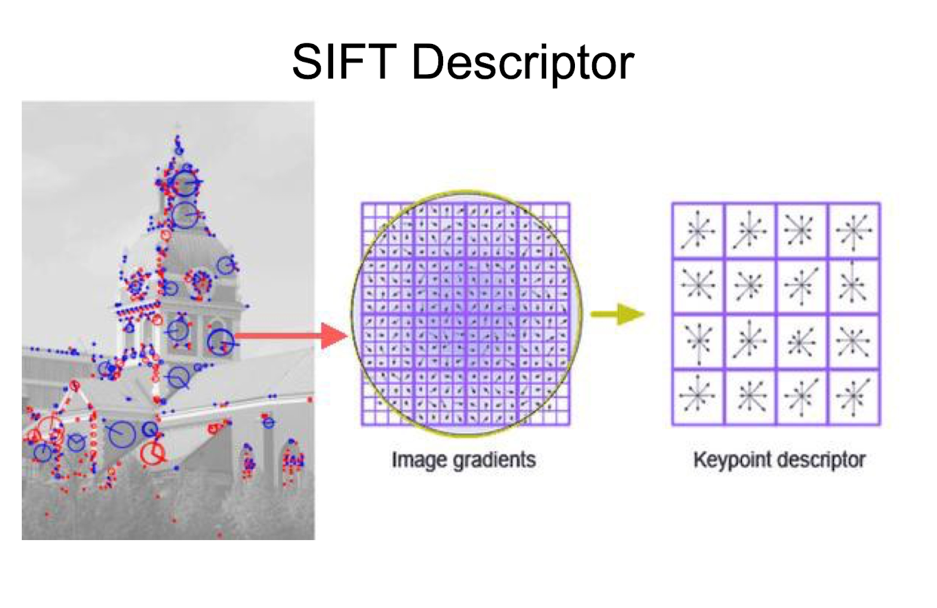
在尺度空间中寻找极值点,并提取出其位置、尺度、方向信息。
Motivation:Harris operator 对尺度不是不变的,而 correlation 对旋转不是不变的。因此需要设计一个对典型观测条件下的变化都鲁棒的 descriptor。
Idea:把图像内容变换到局部特征坐标系中。
1. Scale-space extrema detection
2. Keypoint localization
3. Orientation assignment
4. Keypoint Descriptor
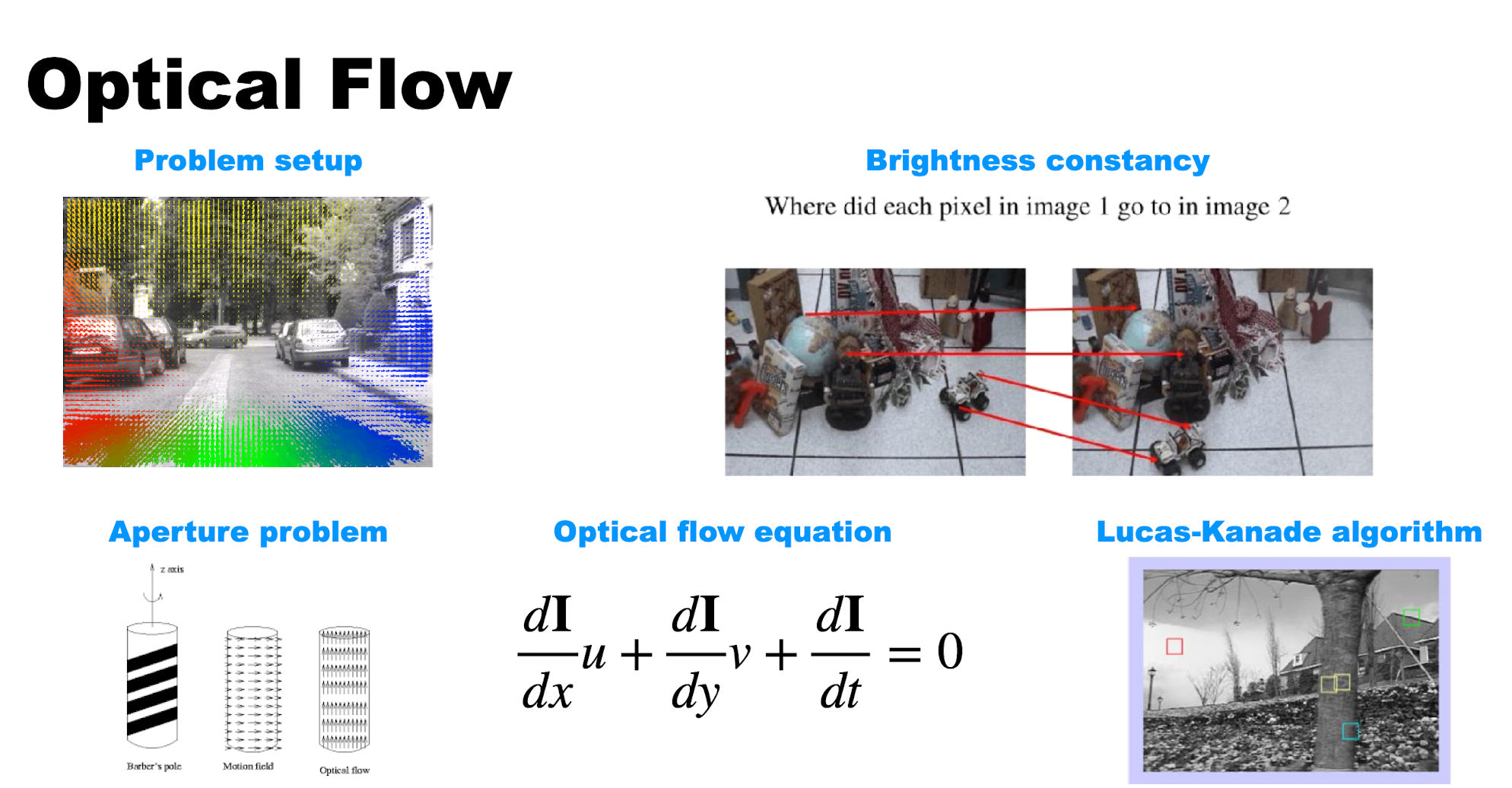
Optical Flow
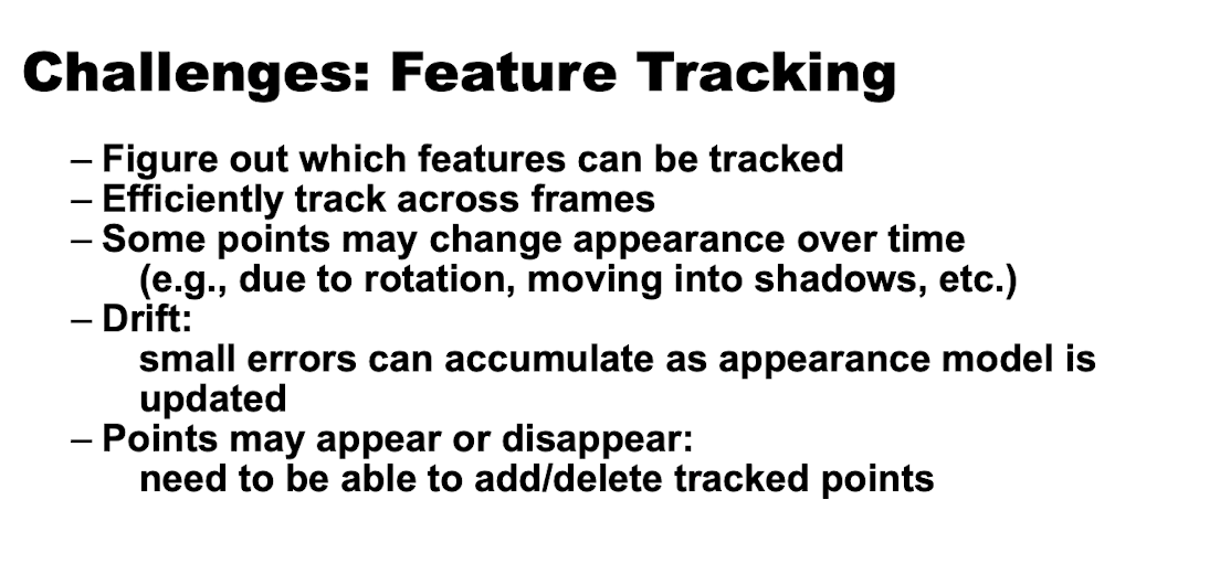
Feature tracking:提取视觉特征(角点、纹理区域)并在多帧上「跟踪」它们。
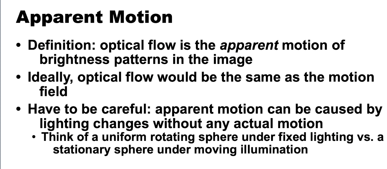
Optical Flow:从时空图像亮度变化中,恢复每个像素处的图像运动。
Feature Tracking
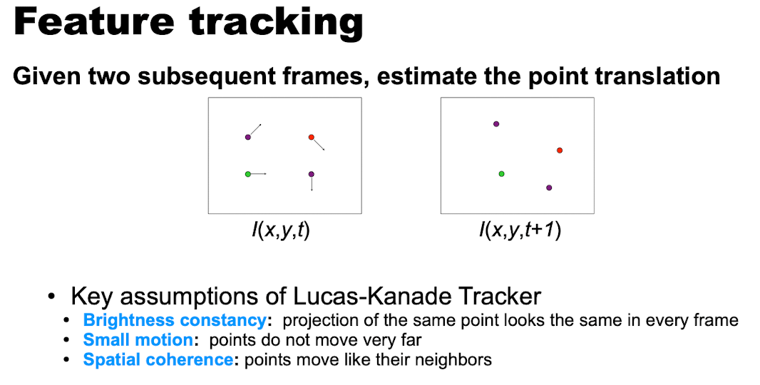
Brightness constancy 推导:
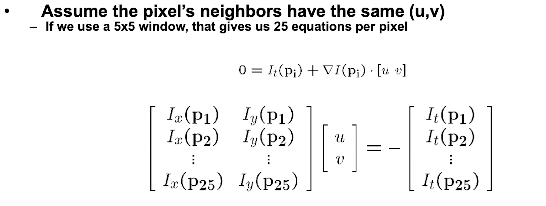
\[ \begin{aligned} &\nabla I \cdot [u,v]^T + I_t = 0 \\ &\nabla I = [I_x,I_y] \end{aligned} \]
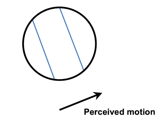
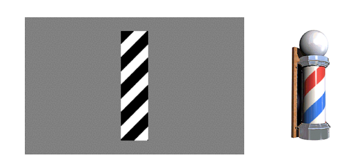
这个式子只能解出运动在亮度梯度方向上的分量。换句话说,它可以告诉我们沿亮度变化方向的运动,但无法告诉我们沿梯度垂直方向的分量——这个问题称为光流的「孔径问题」。
该式子也叫做光流约束方程。
The Aperture Problem
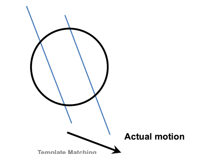
Barber Pole Illusion
Addressing the Ambiguity
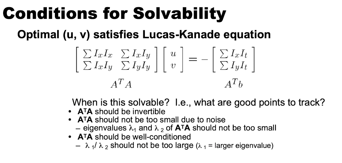

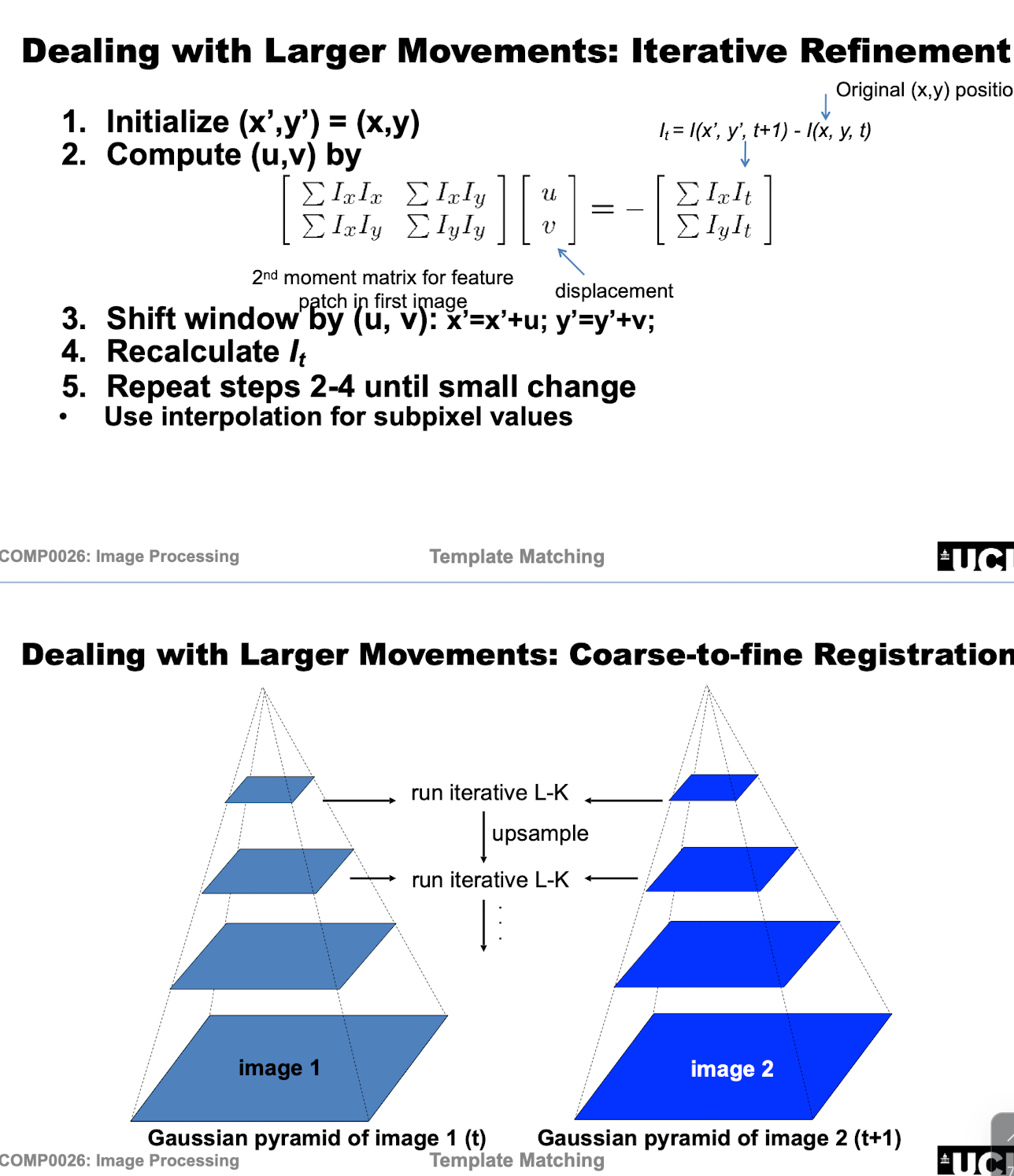
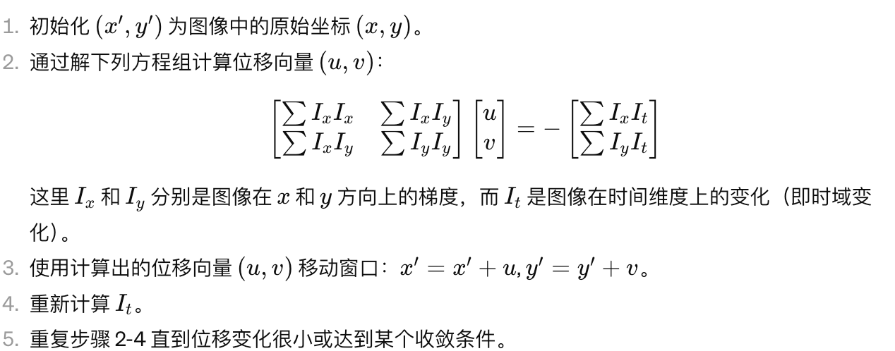
Shi-Tomasi Feature Tracker
\[ R = \min(\lambda_1, \lambda_2) \]
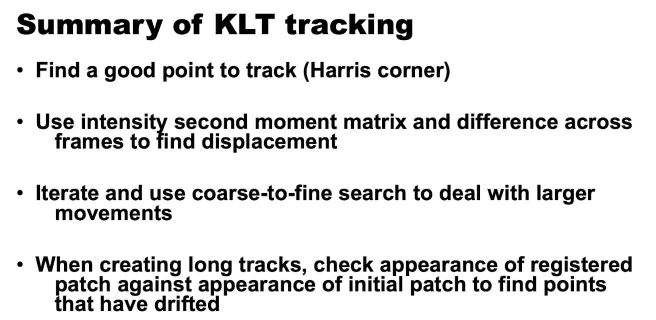
Kanade-Lucas-Tomasi 算法总结
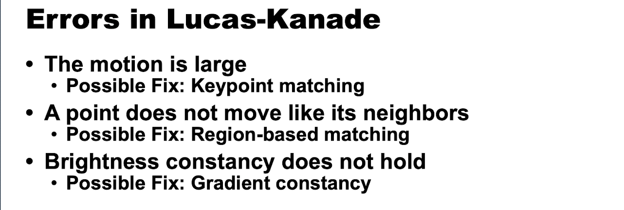
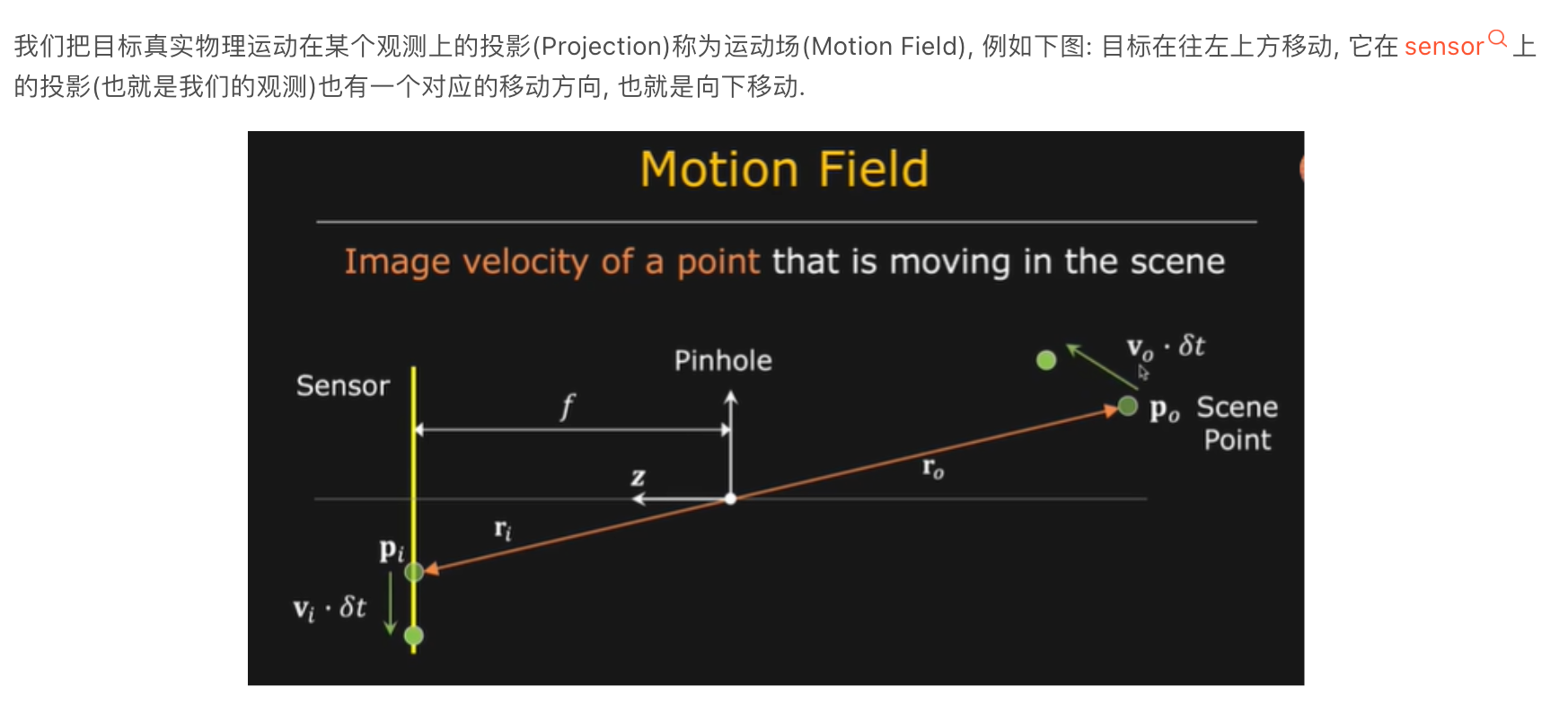
Motion Field
多分辨率 LK 算法