TRELLIS: Structured 3D Latents for Scalable and Versatile 3D Generation
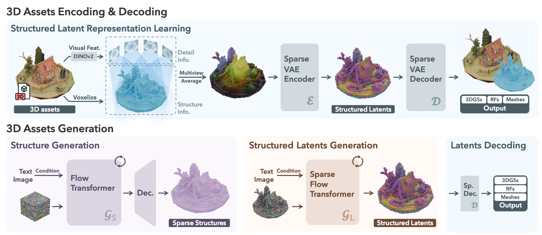
目标是构建一个统一且通用的 latent space,使得高质量 3D 生成可以跨多种表示进行。
- 为了统一:在 latent space 的设计中引入显式的 sparse 3D structure。
- 为了能够生成不同的 3D 表示:给 sparse structure 配上一个强力的 vision foundation model 来编码细节信息——因为它已被证明具有很强的 3D awareness 和细节表达能力。
Structured latent representation
\[ \boldsymbol{z}=\{(\boldsymbol{z}_i,\boldsymbol{p}_i)\}_{i=1}^L,\quad \boldsymbol{z}_i\in\mathbb{R}^C,\quad \boldsymbol{p}_i\in\{0,1,\ldots,N-1\}^3 \]
- \(\boldsymbol{p}_i\) 是与 3D asset 表面相交的 active voxel 在 3D grid 中的位置索引
- \(\boldsymbol{z}_i\) 是附着在对应 voxel 上的 local latent
- \(N\) 是 3D grid 的空间边长
- \(L\) 是 active voxel 的总数
Structured latents 的编码与解码
首先把每个 3D asset \(O\) 转成 voxelized feature \(f = \{(f_i,p_i)\}_{i=1}^L\)。为了得到 \(f_i\),需要汇总来自密集视角的特征:随机 sample 不同相机视角下的图片,用 DINOv2 提取 feature map;每个 voxel 被投影到多视角的 feature map 上,检索对应的特征,然后聚合不同视角下的特征作为最终特征。
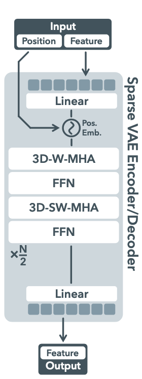
sparse VAE 的 encoder/decoder 结构如下图,两者结构相同,使用重建损失和 KL 损失训练。Decoder 对于不同的 3D 表征结构也是一样的,只是输出略有区别:
- 3DGS:每个 \(z_i\) 被解码成 \(K\) 个高斯,含 position offsets \(o\)、colors \(c\)、scales \(s\)、opacities \(\alpha\)、rotations \(r\)。
- Radiance Fields:使用 Strivec 的思想,把 Radiance Fields 做 CP 分解为张量表示,分别包含空间方向和颜色信息。
- Meshes:FlexiCubes 中的 flexible parameters 和 signed distance values。
事实上是用 3DGS 训练了 encoder 和 decoder,其他表达方式都是 freeze 住 encoder,然后从头训练各自的 decoder。
module 采用了 3D shifted window attention 来促进局部信息交互并提升效率。
Structured latents generation
先 generate sparse structure,然后把 local feature append 上去。
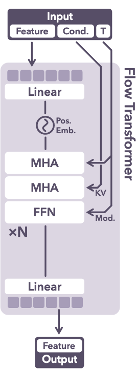
不是直接生成一个 dense binary 3D grid \(O \in \{0,1\}^{N\times N \times N}\),而是先用 3D 卷积 block 把这个 3D grid 编码成一个 low-resolution feature。
然后在这个 low-resolution feature 上训练 \(G_s\)。生成时先生成 low-resolution feature,再通过与 3D 卷积对应的 decoder 变回原来的 3D grid,从而求得 active voxels \(\{p_i\}_{i=1}^L\)。
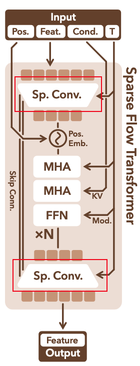
第二个 stage 是生成 latents \(\{z_i\}_{i=1}^L\)。有了 active voxels 之后,就可以通过一个 \(G_L\) 生成。和 DiT 一样,为了提升效率,在 serialization 之前把 input 打包成更短的序列。
Ablation
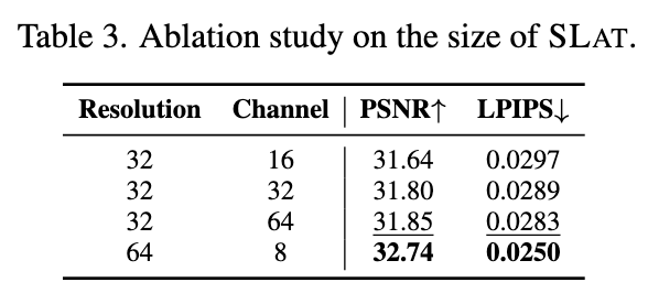
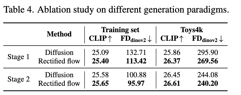
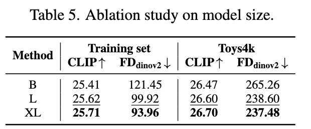
Applications
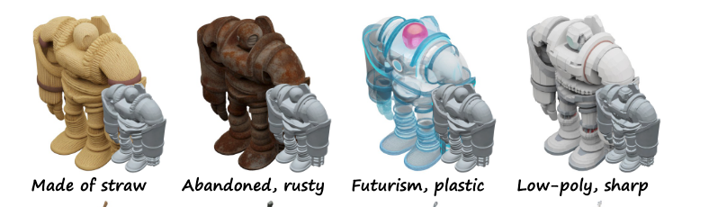
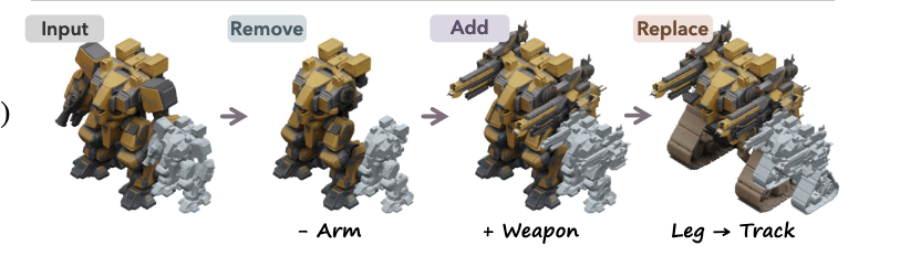
3D asset variations
Region-specific editing of 3D assets(guided by text or images)
Training
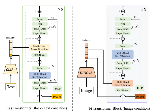
训练中会遇到不稳定的问题,来源是 multi-head attention block 内部 query 和 key 的 norm 爆炸。为了缓解这一点,作者在把 query 和 key 送进 attention 之前先做 RMSNorm。
Limitations
- two stage 的方案不如 one stage 有效
- 没有分离光照效果(does not separate lighting effects)
Code(暂时只开源了 Image-to-3D)
整体可以看成两个 stage:一个是 sparse structure 的生成 stage,包含它的 encoder 和 decoder;另一个是 structured latents 的生成 stage,同样包含它的 encoder 和 decoder。
第一步:preprocess image
对输入图像进行预处理,具体包括检查透明通道、移除背景、裁剪图像到主体区域、调整大小等操作,最终返回一个标准化的图像。
第二步:get_cond
1 | def encode_image(self, image: Union[torch.Tensor, list[Image.Image]]) -> torch.Tensor: |
Sparse Structure VAE encoder architecture
1 | self.input_layer = nn.Conv3d(in_channels, channels[0], 3, padding=1) |
Sparse Structure VAE decoder architecture
1 | self.middle_block = nn.Sequential(*[ |
Structured Latents encoder architecture
1 | super().__init__( |
其中 super():
1 | if pe_mode == "ape": |
其中 SparseTransformerBlock:
1 | self.norm1 = LayerNorm32(channels, elementwise_affine=ln_affine, eps=1e-6) |
其中 SparseMultiHeadAttention:
1 | if self._type == "self": |
其中 SparseFeedForwardNet:
1 | def __init__(self, channels: int, mlp_ratio: float = 4.0): |
Structured Latents decoder architecture(以 GS 为例)
1 | super().__init__( |
Sparse structure flow
1 | # 其他的一些模块处理: |
1 | # input block: |
Structured latent flow
1 | # 其他的一些模块处理: |
1 | # Sp.Conv: (Down block) |
其中 ModulatedSparseTransformerCrossBlock:
1 | self.norm1 = LayerNorm32(channels, elementwise_affine=False, eps=1e-6) |
其中 SparseResBlock3d:
1 | self.norm1 = LayerNorm32(channels, elementwise_affine=True, eps=1e-6) |
DiffSplat: Repurposing Image Diffusion Models for Scalable Gaussian Splat Generation
提出一个轻量的重建模型,能够即时产生 multi-view Gaussian grid,用于可扩展的数据集构建。
用一组结构良好的 Gaussian 2D grid 来表示一个 3D 物体。
在训练阶段,这些 grid 可以在 0.1 秒内从多视角图像中回归出来,从而支撑可扩展的高质量 3D 数据集构建。
DiffGS: Functional Gaussian Splatting Diffusion
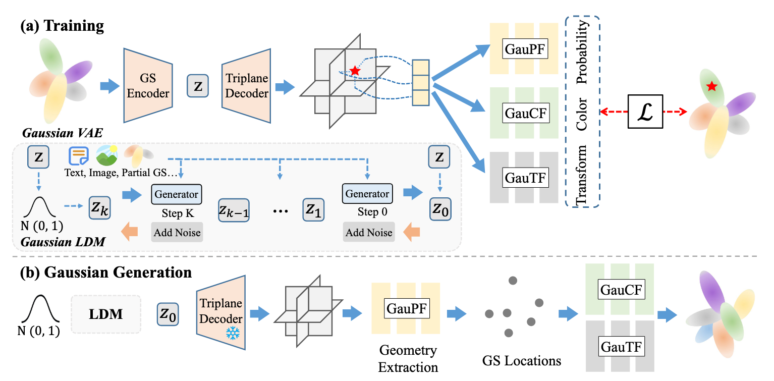
核心思想是把 3DGS 解耦成若干个不同的函数来表示。
Gaussian Probability Function
通过建模每个采样 3D 位置「是一个高斯中心」的概率,来表示 3DGS 的几何:
\[ p_j=\mathrm{GauPF}(q_j)\in[0,1] \]
这个建模思路来自一个观察:一个 3D 位置 \(q_j\) 离所有高斯越远,就越不可能有高斯占据 \(q_j\) 处的空间。
\[ \mathrm{GauPF}(q_j)=\tau\big(\lambda(\min_{i\in[1,N]}\|q_j-\sigma_i\|_2)\big) \]
Gaussian Color and Transform Modeling
\[ \{c_i\}=\mathrm{GauCF}(\sigma_i);\qquad \{r_i,s_i,o_i\}=\mathrm{GauTF}(\sigma_i) \]
Pipeline
给定一个拟合好的 3DGS \(G = \{g_i\}_{i=1}^N\) 作为输入,GS encoder \(\phi_{en}\) 从 \(G\) 中提取全局 latent feature \(z\),再用 decoder \(\phi_{de}\) 解码成一个 feature triplane \(t \in \mathbb{R}^{H \times W \times C \times 3}\):
\[ z=\phi_{en}(G);\qquad t=\phi_{de}(z) \]
然后通过 \(f_j = \operatorname{interp}(t,q_j)\) 得到 3D 位置 \(q_j\) 的特征:
\[ \{\hat{p}_i\}=\psi_{pf}(f_j);\quad \{\hat{c}_i\}=\psi_{cf}(f_j);\quad \{\hat{r}_i,\hat{s}_i,\hat{o}_i\}=\psi_{tf}(f_j) \]
实际训练目标为
\[ \mathcal{L}_\mathrm{VAE}=\big\|\{\hat{p},\hat{c},\hat{r},\hat{s},\hat{o}\}-\{p,c,r,s,o\}\big\|_1 +\beta\, D_{KL}\big(\mathcal{Q}_\phi(z\mid G)\,\|\,\mathcal{P}(z)\big) \]
Dataset Preparation
DiffGS 以拟合好的 3DGS 作为输入来学习生成模型。为了准备 ShapeNet 的 3DGS 数据集,先用 blender 从 ground truth mesh 均匀渲染 100 个视角,得到 ShapeNet 中 chair 和 airplane 两类每个 3D shape 的密集多视角图像;之后用原版 3D Gaussian Splatting 方法,用这些渲染图为每个 shape 拟合 3DGS。
为了得到更稳定、更规整的 3DGS 数据以利于生成建模,作者设计了两个策略:
- 由于是从已知几何的现有 3D 数据集拟合 3DGS,可以直接从表面均匀采样密集点云作为 3DGS 优化的完美初始化,而不必用 COLMAP 点。采样点数设为 100K。
- 观察到自由优化 3DGS 常常会产生一些极大的高斯,这会导致 Gaussian VAE 和 latent diffusion model 训练不稳定,进而影响生成结果。因此把 scale 裁剪到最大 0.01,以避免异常高斯。
Application
- Text/Image-conditional Gaussian Splatting Generation
- Unconditional Generation
- Gaussian Splatting Completion:从存在大面积遮挡的 partial 3DGS 恢复完整的 3DGS。做法是把 partial 3DGS 作为 condition 引入 DiffGS,并用一个改造过的 PointNet 作为 partial 3DGS 的专用 encoder \(\gamma_{partial}\)。
- Point-to-Gaussian generation:给定一个 3D 点云作为输入,生成高斯属性。
Point-to-Gaussian generation 的数据准备
对于 Point-to-Gaussian generation 任务,先把训练/测试数据准备成「点云—3DGS」配对,配对通过 Gaussian Splatting fitting 过程获得。具体来说,点云由在 ground truth mesh 上密集采样 100K 个点得到,配对的 3DGS 则通过用绕 mesh 渲染的多视角图像优化得到。
SAR3D: Autoregressive 3D Object Generation and Understanding via Multi-scale 3D VQVAE
提出一个框架,利用 multi-scale 3D vector-quantized VAE 把 3D 物体 tokenize,以实现高效的自回归生成和细粒度理解。
训练一个自回归模型,基于前面的 scale 来预测 latent triplane 的下一个 scale,并以单张图像或文本 prompt 作为 condition。
Pipeline
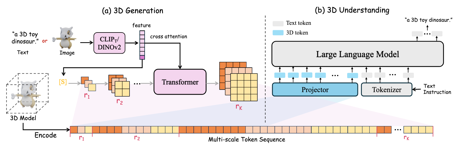
与 Janus 对生成和理解使用不同 encoder 不同,这里只用单一 encoder,分别用完整序列做生成、截断序列做理解。
这篇文章在获取 3D structure 等性质时,使用 RGB、Depth、Plücker Rays map 作为输入送给 multi-view encoder。
模型输入是一张 RGB-D 图像。设 \(I \in \mathbb{R}^{H\times W\times 3}\) 为 RGB 图像,\(\Delta \in \mathbb{R}^{H\times W}\) 为对应的 depth。用 \(\Delta\) 把像素反投影到 3D 中的位置 \(P \in \mathbb{R}^{H \times W \times 3}\)。\(I\) 和 \(P\) 被编码成单一表示 \(R\):
\[ R := f\big(E^{RGB}(I),\, E^{XYZ}(P)\big) \in \mathbb{R}^{N^{enc} \times C} \]
最终特征表示为 \(\tilde{M} = [I \oplus \Delta \oplus P] \in \mathbb{R}^{H \times W \times 7}\)。
为了获得更好的 3D awareness,latent space 被设计成 latent triplane。
Multiscale 3D VQVAE
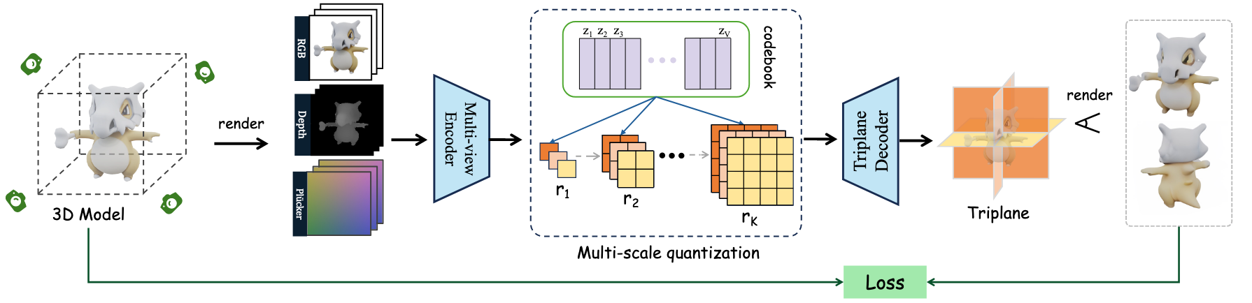
编码之后,\(f\) 被插值到不同 scale,并用 latent triplane quantization layer \(Q\) 量化:
- 输入:原始图像 \(im\),多尺度分辨率 \((h_k, w_k)\)
- 提取特征 \(f = E(im)\),初始化 token 序列 \(R\)
- 对每个尺度 \(k = 1, \ldots, K\):
- 下采样特征图 \(f\) 到 \((h_k, w_k)\)
- 量化生成 token \(r_k\)
- 通过共享码本查找 \(z_k = \operatorname{lookup}(Z, r_k)\)
- 上采样 \(z_k\) 回到最高分辨率 \((h_K, w_K)\)
- 更新残差 \(f = f - \phi_k(z_k)\)
- 输出:多尺度 tokens \(R = (r_1, r_2, \ldots, r_K) \in \mathbb{R}^{3 \times h_K \times w_K \times C}\)
Implementation
与 GaussianAnything(见后文)类似,对于不同的 condition(text 或 image),会交换 Transformer Block 内部的结构。
GaussianAnything: Interactive Point Cloud Latent Diffusion for 3D Generation
一个级联的 latent diffusion model,用于改进 shape-texture 解耦。新提出的 latent space 天然支持几何—纹理解耦,从而允许 3D-aware editing。
这篇探究了此前直接生成 3D 路线中的 latent space——究竟什么才是一个好的 latent space?
- 有使用latent tri-plane 的:不适合交互式 3D 编辑,因为对某一个平面的改动,可能并不对应到需要编辑的那个物体部位。
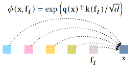
- 也有使用set latent 的(来自 3DShape2VecSet:任何形状都可以用固定长度的 latent 数组表示)。Latent set 通过 cross-attention 机制,在 query 坐标和 anchor 特征之间计算相似性。
但上面的方法都有问题,所以这里使用了一个交互式的 Point Cloud-structured Latent Space。
原文声称:本方案输出的一组高斯均匀分布在 3D 物体表面,Gaussian utilization ratio 接近 100%。
这句话的意思是:在别的方法里,大量预测出来的高斯是「浪费掉」的。用 triplane 或非结构化 set latent 的方法,decoder 要凭空猜每个高斯该放在哪儿,结果相当一部分高斯会飘到空气里、或者堆叠在同一处冗余重复——它们 opacity 接近零,对渲染没有贡献,却占用了表示预算。
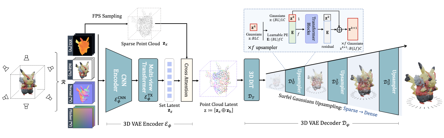
GaussianAnything 之所以能接近 100%,是因为它的 latent 本身就是点云结构:\(\mathbf{z}_x\) 是用 FPS 在物体表面上采出来的点,每个 latent 点带着自己的坐标。decoder 只需要在这些已经位于表面上的锚点附近做局部细化,而不必从零猜位置。于是每个 latent 点都必然解码出一个真正落在表面上、真正参与渲染的高斯。
再加上输出的是 surfel Gaussian(2D 高斯/面元),它天然贴合表面而不是去填充体积,进一步保证了「每个基元都在该在的地方」。
实际收益就是:在同样的基元预算下,表面覆盖更完整、几何精度(Chamfer distance、normal consistency)更高,提取出的 mesh 质量也更好。
Pipeline
Input:不使用密集点云,而采用 multi-view posed RGB-D-N 图像作为输入。这样能更全面地编码 3D 输入,也能被成熟的网络架构灵活高效地处理。所以
\[ \tilde{R} = [I \oplus X \oplus N \oplus P] \in \mathbb{R}^{H \times W \times (3+3+3+6)=15} \]
这里的 multi-view encoder 和 LDM 里面的 VAE encoder 很类似。
第一步:
\[ \mathbf{z}_z=\mathcal{E}_{\boldsymbol{\phi}}^{\mathrm{TX}}\big(\mathcal{E}_{\boldsymbol{\phi}}^{\mathrm{CNN}}(\{\tilde{R}\})\big) \]
其中 \(\mathbf{z}_z\) 是对应 3D 输入的 set latent,它完整捕获了输入所对应的 3D 信息。
但 set latent 不能直接用于 diffusion 学习,因为缺少一个规整的、低秩的 latent space。为了解决这个问题,作者提出 point cloud-structured latent space:通过 cross-attention 层,把非结构化的特征 \(\mathbf{z}_z\) 投影到输入 3D shape 的 manifold 上。其中 \(\mathbf{z}_x\) 是用 Farthest Point Sampling 得到的一些表面点。最终得到 point-cloud structured latent code \(\mathbf{z} = [\mathbf{z}_x \oplus \mathbf{z}_h] \in \mathbb{R}^{(3+C_h) \times N}\):
\[ \mathbf{z}_h:=\mathrm{CrossAttn}\big(\mathrm{PE}(\mathbf{z}_x),\ \mathbf{z}_z,\ \mathbf{z}_z\big) \]
第二步:通过 3D-DiT block 解码输入
\[ \tilde{\mathbf{z}}:=\mathcal{D}_T(\mathrm{MLP}(\mathbf{z})) \]
第三步:通过 transformer block 逐步上采样 latent feature,最后拿最后一个尺度的 tokens \(\mathbf{z}^k\) 去预测 surfel Gaussian 的 13 个参数
\[ \mathbf{z}_i^{(k+1)}:=\mathcal{D}_U^k\big([\mathbf{z}_u\oplus\tilde{\mathbf{z}}_i]\big) \]
Diffusion Process
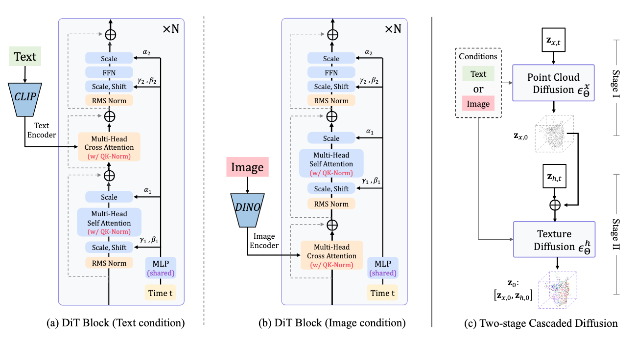
对于不同的 condition(image 或 text),融入的方式不一样,会改变 DiT 架构的顺序。对于生成,分成两个阶段:第一阶段先生成点云,第二阶段再生成 texture,最后用预训练好的 VAE decoder 变成 3DGS。
对于 text condition:使用 CLIP 提取倒数第二层的 token 作为 condition。
Conclusion
SDS 类方法由于 2D diffusion model 中缺乏 3D 信息,难以保持 3D 一致性,这一现象通常被称为 Janus problem。